A Probabilistic View on Reconstruction Losses
In the last article, we expanded our understanding of probabilistic models by understanding linear regression through the probabilistic lens. Now, we will go even further by considering the “reconstruction loss” in (variational) autoencoders (VAEs). The main complexity comes from the usually high-dimensional data, as opposed to the single target variable considered in basic regression tasks.
This post assumes familiarity with VAEs, although the details of that framework are actually not super important to understand the topics discussed here. It also gets quite technical about minor details. If you are reading this because you have been following our LGM class, consider this advanced optional reading for those interested in mathematical details.
Reconstruction Loss in Variational Autoencoders
Recall that we would like to maximize the log probability of the data, $\log(p(x))$, but this is intractable in most latent variable models. Thus, we optimize the variational lower bound instead:
\[\mathcal{L}(x, q) = -D_{KL} (q(z|x) || p(z)) + \mathbb{E}_{q(z|x)}(\log(p(x|z)))\]Here, the left term is the Kullback-Leibler-Divergence between the variational posterior and the prior, and the right part is the log-likelihood of the data. In this article, we want to focus on the latter part.
We have previously seen how to convert abstract probabilities into concrete loss functions we can then optimize. The main step, as before, is to find a suitable distribution $p(x|z)$. There is just one challenge: Previously, we dealt with $x$ just being a single number. But in the case of VAEs, we usually deal with high-dimensional data such as images consisting of many pixels. That is, one datapoint $x_i$ in our dataset is actually a vector of numbers, $x_i = (x_{i1}, x_{i2}, \ldots, x_{id})$ for images with $d$ pixels.1 Accordingly, we need high-dimensional probability distributions over vectors. These can often be complex to evaluate, which in turn makes optimization difficult.
The Independence Assumption
There is one way to side-step the above issue: For two random variables $a$ and $b$, if they are independent from each other, then $p(a, b) = p(a)p(b)$, meaning that the joint probability factorizes. For our image-pixel example, that would mean for an image $x_i$,
\[p(x_i|z_i) = p(x_{i1}, \ldots, x_{id} | z_i) = \prod_j p(x_{ij} | z_i)\]Or in the log case:
\[\log(p(x_i|z_i)) = \sum_j \log(p(x_{ij} | z_i))\]This means that, if we assume independence between pixels given $z$, the (log-)likelihood decomposes into probabilities for each single pixel. And that, in turn, means we can once again focus on probability distributions over just single numbers.
However, you may ask if this assumption makes sense. Intuitively, assuming independence between pixels just seems wrong. In natural images, clearly there are dependencies between different positions. For example, neighbouring pixels tend to be of similar color. There may also be longer-range dependencies, such as in repetitive patterns across an image. However, note that we only require independence given $z$. You can imagine this to mean that the latent variables $z$ are responsible for “coordinating” the distributions over the different pixel positions, such that neighboring pixels are likely to match anyway. Still, the assumption is likely problematic – but it’s also the easiest solution by far.
Choosing a Distribution
In our previous examples, the choice of distribution for our data was relatively straightforward. In the coin flip example, the Bernoulli distribution was a natural choice. In linear regression, the assumption of a Gaussian-distributed error term lead to a Gaussian distribution on $y$, as well. But for image pixels, there seems to be no natural choice. Maybe we just pick something and see what happens?
Gaussian, Fixed Variance
We could just go with a Gaussian again. Does this make sense? Not really: The Gaussian distribution is non-zero over the entire range of real numbers, meaning that for a Gaussian-distributed random variable, technically any value should be possible. Of course, anything more than a few standard deviations away from the mean is near-impossible in practice, so we can often get away with assuming Gaussians where they are technically “wrong”.
But what about the image case? Most often, we represent pixels as being in the range [0, 1]. This is a quite narrow range. What if we want to represent the belief that a certain pixel should be black (represented by the number 0), with a slight chance of being somewhat lighter? We might predict a mean of 0 and assume a small standard deviation. But that would automatically extend our distribution into the negative numbers, since the Gaussian distribution is symmetric.
Still, the practical relevance of this issue is a bit questionable, as we usually just use the mean anyway, and we can easily restrict that into a range either through clipping or a squashing function like the logistic sigmoid. For now, we could just see what happens. In fact, this is exactly the same situation as with the regression model we considered in the last article: Maximizing a Gaussian likelihood with fixed variance is equivalent to minimizing the mean squared error. Thus, if you make the following assumptions:
- Pixel values are independent given $z$,
- Pixels follow a Gaussian distributions with a “global” fixed variance,
then the mean squared error is the correct reconstruction loss for our VAE. Still, it can be instructive to consider other choices.
Bernoulli
If you go and look for VAE code tutorials on the web, you will find many that use the binary (or sigmoid) cross-entropy, among them the official Tensorflow VAE tutorial. Recall from the first post in this series that the binary cross-entropy is what you get as a loss function when assuming a Bernoulli likelihood and apply maximum likelihood:
\[- \log(p(x|\theta)) = - x \log(\theta) - (1-x) \log(1-\theta)\]The Bernoulli likelihood is intended only for binary $x \in {0, 1}$. However, the formula above works perfectly fine for any $x$ in the range $[0, 1]$. Below is a graph of the cross-entropy as a function of $\theta$ (our model output) for various values of $x$ (the data):
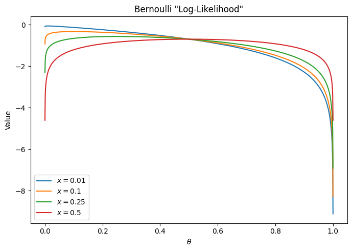
It’s not so easy to see on the graph, but for each $x$, the minimum of the function is at $\theta = x$, and so using this as a reconstruction loss should lead to proper results: It is minimized if and only if the output is equal to the data. And yet, from a probabilistic perspective, this whole thing makes no sense. If our data consists of real numbers in a range, it cannot be Bernoulli-distributed. And simply extending the Bernoulli distribution from binary numbers to the whole range $[0, 1]$ does not result in a probability distribution – it does not integrate to 1. As such, using the cross-entropy for non-binary data is technically invalid.
It looks as though we haven’t really found the ideal reconstruction loss yet. The Gaussian assumption is clearly violated for images, and the assumption of one fixed variance for the entire dataset and all pixels in an image is also questionable. And the Bernoulli assumption is simply invalid. In the remainder of this article, we will look at some attempts to fix these issues. Be warned: This will get quite deep into the nitty-gritty of various probability distributions and should be considered an advanced topic.
Can We Fix It?
Continuous Bernoulli
It seems that we just need a probability distribution defined over the range $[0, 1]$. Then we can derive the log-likelihood and use that for our reconstruction loss. The paper The continuous Bernoulli: Fixing a pervasive error in variational autoencoders does just that. The idea is straightforward: We keep the form of the Bernoulli distribution, but normalize it such that it integrates to 1. This can be achieved by computing the integral over the Bernoulli distribution and then simply dividing by it. The paper claims improved results over the Bernoulli distribution, as well as other valid distributions such as Beta or truncated Gaussian.
Let’s investigate this distribution more closely. Since the continuous Bernoulli (CB) distribution is just Bernoulli multiplied by a normalizer, the log-probability is simply the log-Bernoulli plus the log-normalizer:
\[\log(p(x | \theta)) = x \log(\theta) + (1-x) \log(1-\theta) + \log(C(\theta))\]The form of the normalizer $C(\theta)$ is given in the paper linked above, so please refer to that for details. We can plot the log-normalizer and the log-probability for various parameters $\theta$, and compare it to the incorrectly applied “log-probability” of the standard Bernoulli distribution (see above):
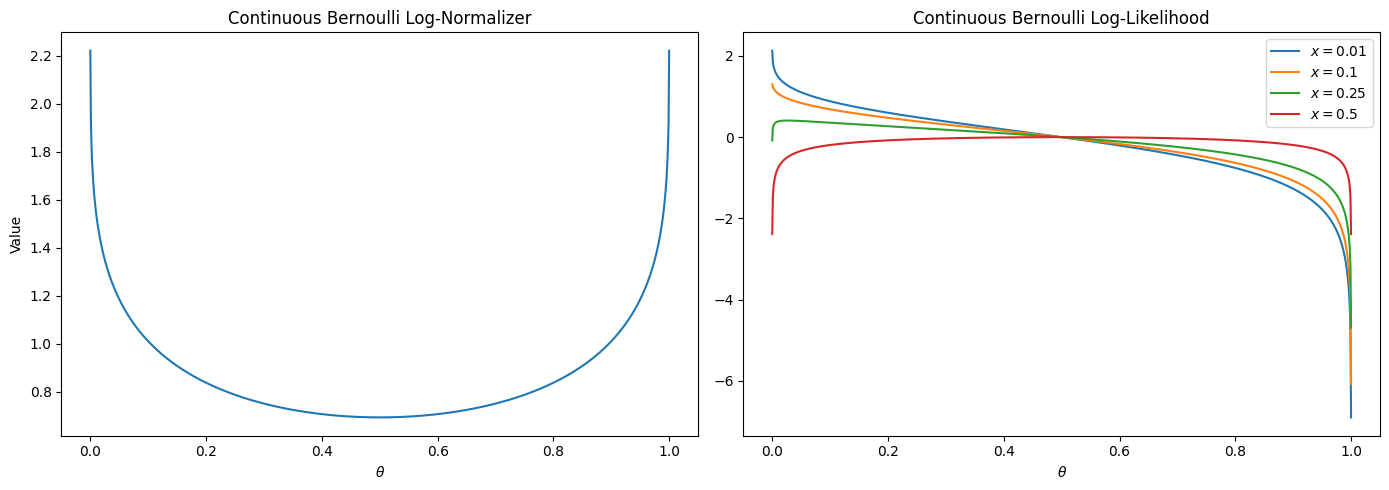
As we can see, the log normalizer increases for the more extreme values of $\theta$. This should push the parameter more towards those values, compared to the standard Bernoulli likelihood. However, for our reconstructions, we usually want to plot the expected values, not the distribution parameters – this is a crucial point we will discuss further below. For the common Bernoulli or Gaussian distributions the expected values are actually just $\theta$ and $\mu$, respectively. That is, they are identical to (one of) the distribution parameters. But for the CB distribution, this is not the case. Here is a plot mapping the distribution parameter $\theta$ to the expected value of the distribution:
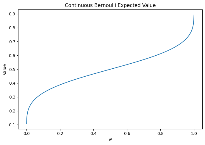
As we can see, the expected value is always less “extreme” (i.e. further away from 0/1) than $\theta$. This means we actually need more extreme $\theta$ values to model any given data point, compared to the regular Bernoulli distribution. As such, this property of the CB distribution is neither good nor bad in itself. Instead, let’s look at some concrete examples to evaluate whether this distribution is actually a good choice.
Sharpness
In section 5.1 of the paper, the authors claim that CB results in sharper images. This would be great, as blurry outputs are a common issue with VAEs. They demonstrate this by plotting the distribution parameters output by the network, not the expected values. Below is a plot that shows how misleading this is. I trained a VAE on MNIST using the CB likelihood. On the left is an image from the dataset, in the middle the “reconstruction” using distribution parameters, and on the right the reconstruction using expected values.
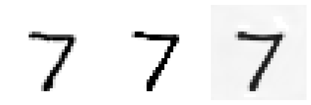
We can see that the supposed sharpness advantage is no longer present when showing the expected values. In fact, the background looks grey instead of white! We will return to this specific issue in a moment. Now you might say, maybe plotting the parameters is just better? But here is the same for an autoencoder trained on CIFAR10:
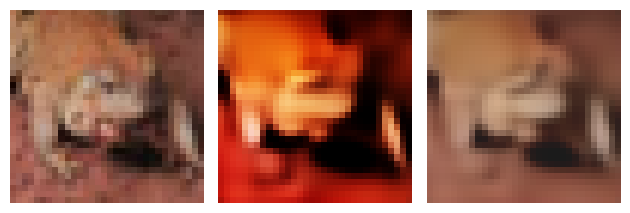
Clearly, the middle image (parameter reconstruction) is extremely oversaturated, whereas the right (expected value reconstruction) seems fine. In the paper, the authors also report results for CIFAR10, but conveniently leave out any reconstruction plots. I find this very fishy, as those would have clearly shown the issue. To me, this raises the question whether the paper is intentionally misleading, or the authors didn’t properly analyse their own models. In fact, you can already see an “oversharpening” of sort in the MNIST image – the reconstruction using the parameter values look sharper than the original, which is not a good reconstruction.
Instability and Color Range
As we have seen above, plotting the distribution parameters as reconstructions is a bad idea. This leaves us with the expected values. However, recall the mapping between parameter and expected value we plotted further above. This function becomes extremely steep near the edge values 0 and 1. This means that, to get an expected value of, say, 0.9, our model needs to output a distribution parameter very close to 1. And what about an expected value of 1, which would be necessary in datasets like MNIST, or any RGB image containing white color? It turns out, this just doesn’t work. The steepness of the mapping means that even tiny changes in $\theta$ lead to huge differences in the expected value. In fact, the code provided by the authors actually cuts off $\theta$ near the edges, as values too close to 1 lead to numerical issues when trying to compute the expected value and log-normalizer. This means it is practically impossible for CB to output images with proper black or white colors. To give you some concrete examples:
- For $\theta=0.9999$ (default choice in the authors’ code), the expected value is merely $0.8915$.
- For $\theta=0.9999999$, the expected value is $0.9373$.
- For $\theta$ even larger, 32-bit numerics fail and we just get an expected value of $1.0$. Also, models trained with $\theta$ allowed to cross this range tend to diverge to infinite loss, since the log-normalizer becomes infinite (at 32-bit precision).
The situation near 0 is symmetric – we either get values nowhere near 0, or the result underflows to a small negative (!) number. This is why, in the plot further above, we see a grey background in the reconstruction, rather than a proper white one. This is no issue for a model trained with standard Bernoulli or Gaussian likelihoods, for example. Here is another example showing a CIFAR image with black & white elements, and the CB reconstruction:
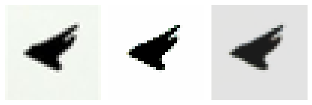
The parameter reconstruction in the middle is overblown, while the expected value reconstruction on the right is too dark.
Comparing FIDs
So, subjective comparison doesn’t look good for the CB likelihood. For completion, I also ran some evaluations using the FID score. I trained simple VAEs on MNIST, keeping all details the same, except for Bernoulli vs. CB likelihood. FIDs were computed using a custom MNIST classifier rather than an Inception network. I also used the beta-VAE framework and tested a range of $\beta$ values. Here are the results:
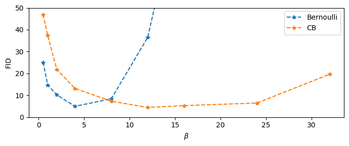
We can see that the results are very similar when controlling for $\beta$. CB likelihood seems to be more robust to a wider range of values, and the best FID reached is actually slightly better than the best one for the Bernoulli likelihood. However, this may well be due to random deviations, as well as insufficient sampling of the $\beta$ space. The main takeaway is that CB likelihood seems to require larger $\beta$. This makes sense: Compared to Bernoulli, CB adds an additional term to the reconstruction loss, which should lead to larger gradients, and thus relatively less impact for the KL-divergence. This, in turn, requires larger $\beta$ to make the KL-divergence more important.
So are these two losses ultimately just “the same”? I would argue no, since the problem of de-saturated images for the CB likelihood remains. The fact that the FID (or the Inception Score, for that matter) doesn’t seem to pick up on this is more of a statement about the blind spots of such measures. At the end of the day, we seem to be left with a rather frustrating conclusion: We can blatantly ignore the limits of our probabilistic framework by using a completely invalid target function (Bernoulli likelihood on a range rather than binary numbers), and yet it seems to work just as well as a different target derived from actual mathematical principles (Continuous Bernoulli). Sometimes, practicality beats correctness.
Of course, we could also probe other distributions over the [0, 1] range, such as the Beta distribution. This one is interesting since it has two parameters $\alpha$ and $\beta$, which generally allows more control over the shape of the distribution. It also makes clear that plotting distribution parameters (as was done in the CB paper) makes no sense, since we have two values for every pixel in this case! The added flexibility can be seen by the fact that the same mean (given by $\frac{\alpha}{\alpha + \beta}$) can be achieved by infinitely many combinations of parameters, as long as the ratio stays the same. Yet, these distributions will have different variances: Generally, larger parameter values will result in smaller variances. This can allow a model to express a measure of “certainty” in the predictions, independent of the expected value. On the flipside, this can get numerically unstable in case of values that are 100% predictable (such as background pixels in MNIST), and requires a few tricks to keep from diverging. Maybe there are more straightforward options with two parameters…?
Revisiting the Gaussian likelihood
Recall the Gaussian log-likelihood:
\[-\log\left(\sqrt{2\pi}\right) -\log(\sigma) -\frac{(x - \mu)^2}{2\sigma^2}\]Previously, we have assumed that $\sigma$ is constant, and after removing constant factors, we were left with the mean squared error. As stated earlier, by assuming conditional independence between pixels, we can then justify applying this loss per pixel. But does this really make sense? Consider a dataset like MNIST. Pixels around the edges are always 0, while others take on varying values. Shouldn’t the edge values be much easier to predict, and thus have a lower standard deviation? This indicates we may want to have a different $\sigma$ per pixel. Also, some images may be easier to predict in general than others, indicating different $\sigma$ values per image. And even if we ignore all that – the constant $\sigma$ assumption was previously useful because it removed the parameter completely from our equations. Does this still hold for VAEs? No!
Recall that for a VAE, we add the KL-divergence to the reconstruction loss, which in turn is the negative log-likelihood. As you can see above, the squared difference is scaled by $\sigma$. But the KL loss is not! This means that, if we just ignore $\sigma$, we are basically forcing a specific relative scale between reconstruction and KL losses. It is in fact similar to setting the $\beta$ value on the KL loss in $\beta$-VAEs. You can imagine it like this: By removing the multiplier $2\sigma^2$, we have basically assumed this value is 1. This implies $\sigma^2 = 0.5$ or $\sigma = \sqrt{0.5} \approx 0.7$. That is, our model assumes a fixed standard deviation of around 0.7 for all pixel predictions. Doesn’t this seem excessively large for values ranged between 0 and 1?
But it gets worse: Scaling images in [0, 1] seems arbitrary. What if we decided to scale them in [0, 255]? Suddenly, a standard deviation of 0.7 is tiny! Note that a smaller $\sigma$ corresponds to a larger squared error, which makes the reconstruction loss more important relative to the KL-loss. All this implies that, even if we are okay with $\sigma$ being a single constant value, at the very least we have to tune it properly. Let’s consider some options for treating $\sigma$. I also recommend the paper on $\sigma$-VAEs, where some of these ideas come from.
- Leave it as a single fixed value that we tune by hand. This is equivalent to $\beta$-VAE.
- Have one fixed value per data dimension (e.g. pixel). This adds flexibility, but seems practically infeasible. Nobody wants to set thousands (or millions) of $\sigma$ values per hand.
- Use either of the above options, but have $\sigma$ be a learnable parameter. By analyzing the log-likelihood, you can see that there are two opposing factors: Maximizing $-\log(\sigma)$ pushes $\sigma$ to be as small as possible. On the other hand, the squared error pushes $\sigma$ to be as large as possible. These two factors will “meet in the middle” somewhere, depending on the value of the squared error.
- Use either of the first two options, but compute $\sigma$ from the data.
All these options have in common that they will use the same $\sigma$ values for all data points (e.g. images). This is somewhat limiting: Remember that our model outputs a probability distribution per data point, so we could use different $\sigma$ values for each example! The most straightforward way is to have $\sigma$ be another output of our model, along with $\mu$. This is easy to implement, and can be trained via backpropagation just like the values for $\mu$. Once again, we can either output a single $\sigma$ per image, or one per data dimension (pixel). For making predictions, $\sigma$ can simply be discarded, and $\mu$ used as output as usual. Thus, adding $\sigma$ as another output only affects the computation of the loss.
Given that $\sigma$ is in some sense a “secondary” parameter (only used for training), we can even take another approach. Namely, we can ask ourselves what the best value for $\sigma$ would be given a specific prediction for $\mu$. Once again there are different cases, such as one $\sigma$ per image, or one per pixel. Let us first look at the latter case – one value per pixel, or generally per data dimension. Here is the full per-dimension loss, which is just the negative log-likelihood:
\[\log\left(\sqrt{2\pi}\right) + \log(\sigma) + \frac{(x - \mu)^2}{2\sigma^2}\]The left term can be discarded since it’s constant, leaving us with
\[L = \log(\sigma) + \frac{(x - \mu)^2}{2\sigma^2}\]To find the optimal value for $\sigma$, we can go the usual route: Compute the derivative, set to 0, and solve. the derivative is
\[\frac{dL}{d\sigma} = \frac{1}{\sigma} - \frac{(x - \mu)^2}{\sigma^3}\]Setting this to 0 and solving for $\sigma$ gives
\[\sigma^2 = (x - \mu)^2\]So the optimal variance, is just the squared distance from the mean, which makes sense. Now we can insert this into the loss above to remove $\sigma$ from the equation:
\[L = \log(|x-\mu|) + \frac{1}{2}\]It turns out, the terms on the right cancel out, since both are just the squared difference! We can of course remove the constant, leaving us just with $\log(|x-\mu|)$. For high-dimensional data such as images, we would simply compute this loss per-element and sum up, as we have seen in the beginning of this article. Here is a plot of this function:
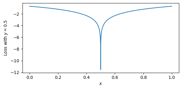
There are a few things to note about this loss function. For one, since $\log(0) = -\infty$, this loss does not have a proper minimum. Rather, it will keep decreasing as the difference gets closer to 0, eventually becoming infinite. This is obviously a problem for actual implementations. In practice, we need to set a lower bound on the variance to prevent this. This loss also has the property that the gradients become larger as the difference gets closer to 0. Essentially, this means that the better a specific value is predicted, the stronger the “pull” will be to predict it even better. Intuitively, this corresponds to reducing the variance of the Gaussian to concentrate it more and more on one point (the mean), which will make it ever more “peaked” and increase the probabilities close to the mean. This property is somewhat opposite to the squared loss, where the gradient (and thus the pull towards a specific value) becomes smaller the closer you get to the target value.
Is this good or bad? I’m not sure. But I personally have not been able to train models with this loss function. It’s simply too unstable. As soon as just one pixel in an image can be predicted near-perfectly, the process seems to diverge, even with a lower bound on the variance. And this is a very simple condition to meet for datasets like MNIST with pixels that are always background.
We could look at a slightly different model, namely one where we have just one $\sigma$ for an entire image. Here, we cannot look at single-pixel losses individually, since $\sigma$ is shared over pixels. However, we can at least keep the assumption of independence between pixels. This implies a Multivariate Gaussian with diagonal covariance matrix. The likelihood looks like this:
\[\frac{1}{\sqrt{2\pi}^d \sigma^d} \exp\left(-\frac{||x-\mu||^2_2}{2\sigma^2}\right)\]Here, $x$ and $\mu$ are now entire vectors, and $||\cdot||^2_2$ denotes the squared euclidean norm, i.e. sum of squares. $d$ is the dimensionality of the data, e.g. number of pixels. Now, the steps are the same as before. Compute the negative log-likelihood and remove constants to get a loss function:
\[L = d\log(\sigma) + \frac{||x-\mu||^2_2}{2\sigma^2}\]Compute the derivative with respect to $\sigma$:
\[\frac{dL}{d\sigma} = \frac{d}{\sigma} - \frac{||x-\mu||^2_2}{\sigma^3}\]Setting this to 0 and solving for $\sigma$ now gives
\[\sigma^2 = \frac{||x-\mu||^2_2}{d}\]Since the numerator is the sum of squared differences from the mean, this is just the mean squared error! We end up in much the same situation as before, where the two terms on the right of the loss function cancel out, and we are left with
\[L = d \log\left(\frac{||x-\mu||_2}{\sqrt{d}}\right)\]The expression in the logarithm is the “root mean squared error”. Some further simplification of these terms and removing constants gives us
\[L = \frac{d}{2} \log\left(||x-\mu||_2^2\right)\]$\frac{d}{2}$ is a constant, but recall that we need to keep multiplicative constants in VAEs to properly scale the reconstruction loss vs. the KL-Divergence. All in all, this loss is similar to the one where we used one $\sigma$ per data dimension. However, the logarithm is applied to the sum of squares, rather the dimension-wise absolute difference. This change makes for a much more stable loss, since we are less likely to have differences near 0 for an entire image, compared to just single values.
I have not tested this loss function extensively, but good pretty good results from small test on FashionMNIST. The property of gradients becoming stronger as predictions become better takes some getting used to, and I still needed to tune $\beta$ for the $\beta$-VAE framework, contrary to what the paper claims.
Conclusion
This was a long one. To summarize:
- We saw how to construct reconstruction losses for (variational) autoencoders by deciding on probability distributions for our data and following the same approaches we have seen in previous articles.
- We learned how assuming conditional independence between data dimensions leads to simple element-wise loss functions.
- Finally, we investigated the questionable assumptions behind commonly used loss functions, and looked at some potential remedies, such as the Continuous Bernoulli distribution, or modeling $\sigma$ in Gaussian distributions.
Unfortunately, it doesn’t look like there is a definite answer for what is the best loss function. Like so often, a paper introducing a new function somehow always shows that this is the best one, but trying to reproduce those results in different contexts is a different story. We have also seen that “incorrect” functions like the binary cross-entropy or squared error can lead to acceptable results.
Still, if we really want to understand generative models deeply, including the theory, these are topics we need to deal with. There doesn’t need to be a correct answer at all; what matters is that we learn how to find and investigate potential new solutions! I hope this mini-series was helpful in doing that. There may be more articles in the future on other topics related to our Generative Models class. See you there!
-
Wherever we talk about images in this article, you could insert any other high-dimensional data structure instead. ↩