A First Look at Probabilistic Modeling
This will be the first in a series of posts I will be writing to accompany our Learning Generative Models class in the winter semester of 2025. Although this is far from the first time we teach this class, I thought this would be a good place to put more detailed explanations that people may want to review later, as well as advanced concepts we don’t have time for in the class itself.
In this post, we will first look at what probabilistic modeling actually is, by considering the example of a coin flip. In the next one, we will then look at linear regression through the probabilistic perspective.
Flipping Coins
Consider what happens when you flip a coin. You throw it, it flips around a few times in the air, and lands either heads or tails up. Now, what if I asked you to predict which side is going to land up? Most likely, you will just make a guess, and you expect to have a 50% chance to be correct (assuming the coin is fair). You would probably say that the result is “random”. But what does that mean?
Probabilities as Abstraction
The coin flip process seems pretty simple to understand. When you throw it, a certain side is showing up. Let’s say heads. While in the air, it will flip a few times. If it doesn’t flip at all, it will land heads up. If it flips once, tails up; twice, heads up; thrice, tails up, etc. It seems all we need to know to “predict” the result is a) which side is up before the throw, and b) how many times the coin will flip while in the air.
Now, I’m no physicist, but it sounds like this should be possible. Given exact information about the force behind the throw, the “angular momentum” of the coin, maybe air resistance etc., we should be able to derive how many times the coin is going to flip, and thus perfectly predict the result. I would think that it’s possible to build a “coin flipping machine” that would always produce a coin flip with the desired outcome. There is really nothing “random” about this!
And yet, this is clearly not feasible for a human, looking at another human flipping a coin. There are too many factors interacting in too complex of a way. And so we make the abstraction of saying that the flip is essentially random, even though this is not really true – it’s just a lot more manageable as well as practically useful.
As such, we create a probabilistic model of the coin throw: We assume that there is some probability $\theta$ that it will land heads up, and accordingly it will land tails up with probability $1-\theta$1. If we denote heads by the number 1 and tails by 0, this can be summarized via the following expression:
\[p(x) = \theta^x (1-\theta)^{1-x}\]This is called the Bernoulli distribution for binary numbers. If the coin is fair, we expect $\theta = 0.5$. This extremely simple model fully describes our abstraction of the coin flip process.
Learning About the World With Models
Once we have a model of some real-world process, we can use it to learn about the world. Let’s say we are playing a coin flipping game, where I flip the coin, and you have to guess the outcome for the possibility of a reward. Now, assuming that I haven’t mastered the art of coin flipping to the degree mentioned earlier, this is simply a guessing game. However, what if the coin is not fair? That is, the coin might land heads up with a probability $\theta \neq 0.5$. Long term, this will skew the results and might throw off your guessing. Let’s say you get suspicious and start tracking the results. After $n$ throws, we got $k$ heads, and $n - k$ tails accordingly. Intuitively, you would probably say that if $k / n$ is too far from 0.5, you conclude that the coin is not fair. But can we formalize this somehow?
Maximum Likelihood
We could say that we want to find the best model given our observations. But what is “best”? One way to formalize this is using probability theory: We want to find $\arg\max_\theta p(\theta | X)$, where $\theta$ represents our model (in this case, just one probability) and $X$ our data (a collection of many coin flips). What exactly we mean by “probability of a model” is a bit of a philosophical topic and beyond our scope here, but we can take it to mean “how much do we believe this model is true”, or just some kind of “score” for the model. That is, we want to find the model with the highest score or believability. Now, Bayes’ rule tells us that
\[p(\theta | X) = \frac{p(X | \theta)p(\theta)}{p(X)}\]We seemingly made the expression more complex – we replaced one probability by three! However, because we only care about which $\theta$ is the best, and not the actual value, we can disregard $p(X)$, as this is just a constant multiplier:
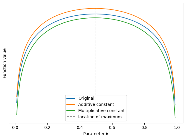
\[p(\theta | X) \sim p(X | \theta)p(\theta)\]Here is a graph showing a function shifted or scaled by a constant – note how the maximum remains at $\theta = 0.5$:
In the equation above, $p(X | \theta)$ is called the likelihood, and $p(\theta)$ the prior. The prior basically gives our beliefs about the model before we have seen any data. For example, we may assume that the coin is probably fair, because most coins are. Then, the prior would be larger for values of $\theta$ around 0.5. For simplicity, we will assume a uniform prior, i.e. $p(\theta) = c$ for some constant $c$. Then, the prior is also just a constant multiplier, and we are left with the likelihood $p(X | \theta)$ as the target to maximize:
\[p(\theta | X) \sim p(X | \theta)\]Since this is called the likelihood, and we want to maximize it, this procedure takes the name maximum likelihood.
Deriving a Solution
Let’s find the optimal $\theta$. To start with, our data $X$ consists of many coin flips $x_1, x_2, \ldots, x_n$. These coin flips are independent, that is, the result of one flip does not influence the next. They are also identically distributed, i.e. $\theta$ is the same for all flips. Since probabilities of independent events factorize, we get
\[p(X | \theta) = \prod_i p(x_i | \theta)\]This is great, because it allows us to think just about probabilities of single coin flips. As we have described further above, these follow a known distribution, the Bernoulli distribution. Unfortunately, the above expression is not quite usable in practice, since it involves a product over potentially many numbers, quickly leading to numerical issues. Thus, we usually work with the log-likelihood instead:
\[\log\left(\prod_i p(x_i | \theta)\right) = \sum_i \log(p(x_i | \theta))\]The fact that the logarithm of a product is the sum of logarithms allows us to avoid multiplying $n$ numbers. And as it turns out, log probabilities often have a simpler functional form, as well. Now we are at a point where we can insert the Bernoulli distribution:
\[\begin{aligned} \sum_i \log(p(x_i | \theta)) &= \sum_i \log(\theta^x_i (1-\theta)^{1-x_i})\\ &= \sum_i x_i\log(\theta) + (1-x_i) \log(1-\theta) \end{aligned}\]Our goal is to find the parameter $\theta$ which maximizes this expression. Recall from calculus that a necessary condition for a maximum is that the derivative is 0 at that point. Thus, we can compute the derivative, set it to 0 and solve for $\theta$. The derivative is given by
\[\sum_i \frac{x_i}{\theta} - \frac{1-x_i}{1-\theta}\]Earlier, we assumed $k$ heads in our data and thus $n-k$ tails. $x_i$ is 1 for heads and 0 for tails, and $1-x_i$ is 1 for tails. Thus, the sum simply evaluates to
\[\frac{k}{\theta} - \frac{n-k}{1-\theta}\]Setting this to 0 gives
\[\frac{k}{\theta} = \frac{n-k}{1-\theta}\]Solving this for $\theta$ is slightly annoying, and there are different ways to do this. Here is one:
\[\begin{aligned} \frac{k}{\theta} &= \frac{n-k}{1-\theta} \\ \iff \frac{\theta}{k} &= \frac{1-\theta}{n-k} \\ \iff \frac{\theta}{k} + \frac{\theta}{n-k} &= \frac{1}{n-k} \\ \iff \frac{\theta(n-k+k)}{k(n-k)} &= \frac{1}{n-k} \\ \iff \frac{\theta n}{k} &= 1 \\ \iff \theta &= \frac{k}{n} \end{aligned}\]Thus, the optimal $\theta$ is just the proportion of heads we saw, which is most likely the intuitive solution you would have come up with anyway! Note that technically, we would still have to check whether this is really a maximum (e.g. using the second derivative). We would also have to treat $k=0$ or $k=n$ as special cases (since we would be dividing by 0 above). However, we will skip these details here.
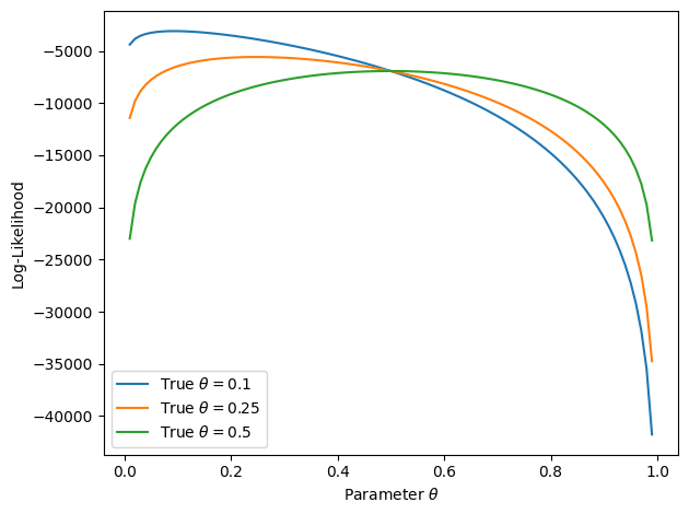
That the point we found is indeed a maximum can be seen when plotting the log-likelihood. For the graph below, we created random data that is 1 with a certain probability $\theta$, and 0 otherwise. For each graph, we use different $\theta$ and do 10,000 flips. We only show $\theta \leq 0.5$ since probabilities larger than 0.5 would look symmetric. For example, the likelihood for $\theta=0.9$ is a mirrored version of $\theta=0.1$.
Advanced Considerations
Revisiting the Prior
Remember that earlier, we simply disregarded the prior on $\theta$. What if we want to include it? Turns out that’s pretty simple. For our target, we would be left with
\[\log\left(p(\theta) \prod_i p(x_i | \theta)\right) = \log(p(\theta)) + \sum_i \log(p(x_i | \theta))\]That is, we simply have to add the log prior. We of course have to choose a distribution; this is a topic going way beyond our scope. However, given that this has to be a distribution over $\theta$, which is a probability, this should be a distribution over the range [0, 1]. A common prior for Bernoulli likelihoods is the Beta distribution. This has
\[\log(p(\theta)) = (\alpha-1)\theta + (\beta - 1)(1-\theta) - B(\alpha, \beta)\]where $B(\alpha,\beta)$ is the so-called Beta function and $\alpha, \beta$ are distribution parameters. In fact, they are hyperparameters that shape the prior on our parameter $\theta$. We will have to choose these appropriately.
This seems complicated. But: When taking the derivative with respect to $\theta$, the Beta function disappears completely, since it is independent of $\theta$. What we are left with then looks a lot like our previous log-likelihood! It turns out a Beta distribution with given $\alpha, \beta$ is equivalent to seeing $\alpha-1$ many heads and $\beta-1$ many tails. For example, if we set $\alpha = \beta = 501$, that is the same as having seen 500 heads and tails before ever having seen any actual data. This reflects a relatively strong prior belief that the coin is fair, and we would need to see a lot more data to convince us otherwise. For example, say you did 1000 flips and saw 800 heads and 200 tails. The maximum likelihood solution would then be $\theta = 800/1000 = 0.8$. But with the aforementioned prior, it would be $1300/2000 = 0.65$.
Connecting to Machine Learning Concepts
Let’s look again at our log-likelihood: $ x_i\log(\theta) + (1-x_i) \log(1-\theta)$. If you put a minus in front of this, what do you get? It’s actually the binary cross-entropy, the loss function you would likely choose when training a neural network on a binary classification problem (e.g. using a single sigmoid output). It turns out the concepts discussed here work in the same way if you replace the fixed $\theta$ by the output of a neural network. Thus, the choice of binary cross-entropy as a loss function is not arbitrary; it corresponds to the maximum likelihood solution!
One fine difference you may have noted is that we are usually averaging over examples for our loss functions, whereas here we are summing. But that isn’t really an issue, since the average is just the sum divided by the number of examples – a constant multiplier! Thus, the solution doesn’t change whether we are summing or averaging.
We can also understand the prior from a different perspective: $ \log(p(\theta)) + \sum_i \log(p(x_i | \theta))$. On the right, we have the “loss function” for our data. On the left we are adding a term independent of the data, only dependent on the model. This is a regularizer! See it the other way: By adding, for example, a weight penalty on a loss function, you are encouraging smaller weights. You are basically expressing a prior belief that the “correct” model has small weights, with the size of the regularization parameter determining the strength of your belief.
Conclusion
This was a first look at understanding data and models through a probabilistic lens. To summarize:
- Real-life processes may be modeled as abstract probabilistic processes.
- Given some data, we can look for the model that best fits our observations.
- A principled way to find a good model is using maximum likelihood, optionally including a prior.
We will expand upon these concepts in the class. For many generative models, it is possible to implement and work with them without having a solid grasp of what is actually going on in the background. But for a Master’s level class, we should aim for a higher level of understanding, and these concepts form the basis. Review them as necessary and clarify doubts in class! In the next post, we will understand linear regression as a probabilistic model, as well. See you there!
-
We will disregard the possibility of the coin landing on the edge. ↩