Linear Regression as a Probabilistic Model
Last time, we looked at how to construct probabilistic models for simple processes such as a coin flip. Such models provide a good basis for understanding, as the involved concepts are fairly intuitive. They are, however, not very useful due to their simplicity. Therefore, we will now understand linear regression as a probabilistic model, as well. This will serve as an introductory example to more complex and abstract models.
Linear Regression
In regression, we generally have some data for so-called independent variables $x$ and dependent variables $y$, with $y$ assumed to somehow depend on $x$. In linear regression, this dependency is assumed to be… linear:
\[y = wx + b\]To be precise, this is an affine-linear model: The input is multiplied by some weight $w$, resulting in the typical straight line, but the line can be shifted away from $(0, 0)$ by the bias $b$. As an example, let’s consider the relation between a person’s height $x$ and weight $y$. Clearly, taller people tend to be heavier on average. It’s not so important whether this relation is really linear – we will just assume that it is so we have an example.
So let’s say we assume a linear relationship, but we don’t know what exactly that relationship is. That is, we don’t know $w$ or $b$. Just like with our coin flip example, we can go and collect data – in this case, this would mean finding a bunch of people and measuring their height and weight. This gives us height data $X$ and weight data $Y$. Then we could define a loss function that measures the difference between model predictions and the true values, and minimize that function. Done! A suitable loss function may be the squared error. But why? Why not the absolute error? Why not some kind of cross-entropy measure? Or something completely different?
Also, the linear model clearly doesn’t explain everything: What about two people who are the same height, but different weight? Clearly, there are other factors at work, so our model cannot be correct. We could try and collect a host of other influences (such as age, gender, ethnicity, physical activity, nutrition…) and include all these in our model. This would significantly complicate the process. Or we once again fall back on abstraction!
Linear Regression With a Random Component
Just because there are other factors influencing weight besides height, that doesn’t mean the relationship between the two variables isn’t linear. We just need a way to conveniently summarize all these other influences. We can do this just like in our coin flip example – by assuming they are essentially random. This means the proper linear regression model is actually
\[y = wx + b + \epsilon\]where $\epsilon$ is a random variable that summarizes all the influences on weight besides height. To have a proper model, we still need to specify what distribution $\epsilon$ follows. By far the most common pick for linear regression is to say that $\epsilon$ follows a Gaussian (or Normal) distribution with mean 0 and some unknown but fixed standard deviation $\sigma$. We write $\epsilon \sim N(0, \sigma)$. In practice, this means that, if I collect tons of weight data for people of the same height, the distribution should be a Gaussian bell curve around some mean value.
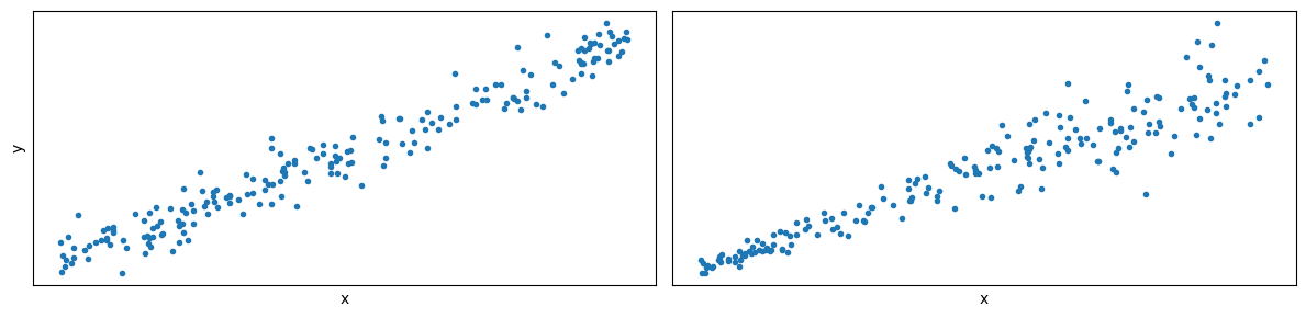
Crucially, the assumption of a fixed $\sigma$ means that this bell curve should have the same spread for all heights. Whether this is true in our example is questionable, and it’s likely that linear regression has been applied to many problems without really checking for this assumption! To illustrate, consider the two plots below: On the left, the assumption of fixed variance is fulfilled. On the right, it’s not – the spread of the data differs along the x-axis.
Next, note that we can actually rewrite $y$ as a random variable:
\[y \sim N(wx + b, \sigma)\]This means that $y$ follows a normal distribution with mean $wx + b$. This formulation is equivalent to the one with adding a 0-centered $\epsilon$. Now we can see that this kind of linear regression is a probabilistic model!
You might say that this seems problematic, as we don’t want to make random predictions about our data. But we don’t have to! In practice, we usually just predict the mean, i.e. $wx + b$. You can actually justify this mathematically, as well. Namely, we want to make the best prediction given our model, and it turns out that the mean is in fact the best prediction under certain assumptions about what “best” means. For example, we might want our prediction to minimize the expected squared error between itself and the true (random) value.
Finding the Best Model
Crucially, the formulation as a probabilistic model gives us a principled way to approach finding the best parameters. Since we went through these steps for the coin flip example in the las post, we will not repeat them here. However, we can once again apply the maximum likelihood principle (or optionally add a prior).
The actual equations are slightly more complicated, because now we have both $X$ and $Y$ for data. Most importantly, we are no longer directly optimizing the parameters of our probability distribution, as we did with $\theta$ for the coin flip. Rather, the mean of our normal distribution is the output of an affine-linear function, which in turn has its own parameters $w$ and $b$! This is much closer to the models we will see in this class. However, right now we will still consider the distribution parameters $\mu$ and $\sigma$ directly. If we went through the derivation again, we would eventually end up with the formula for the log-likelihood of the dataset:
\[\sum_i \log(p(y_i | \mu_i, \sigma))\]Note that we have written $\mu_i$ to denote that the mean is different for each data point, since it is the result of our linear model applied to $x_i$. Now we just have to insert the logarithm of the normal distribution:
\[\sum_i -\log\left(\sqrt{2\pi}\right) -\log(\sigma) -\frac{(y_i - \mu_i)^2}{2\sigma^2}\]Earlier, we assumed that $\sigma$ is constant. That means we only need to optimize for the mean $\mu_i = wx_i + b$. Since adding constants doesn’t change the optimization results, we can remove them:
\[\sum_i -\frac{(y_i - \mu_i)^2}{2\sigma^2}\]After removing the additive constants, $2\sigma^2$ is now a lone multiplicative constant, which we can also remove. So we are left with
\[\sum_i -(y_i - \mu_i)^2\]Recall that this is the log-likelihood we want to maximize. If we were to use a setup where we have a loss to minimize, we could simply remove the minus and minimize
\[\sum_i (y_i - \mu_i)^2\]It’s the sum of squared errors! Thus, it turns out this loss function is not arbitrary. Optimizing the sum of squares corresponds to maximum likelihood for a model with Gaussian likelihood and a fixed, constant $\sigma$.
Did that really help us? We wanted to use the squared error anyway! However, we gained two things:
- We understood the assumptions implied by using squared error.
- We could now construct regression models with non-Gaussian errors and derive appropriate error functions.
The second point is particularly relevant in cases where we have a principled reason to assume specific random components, e.g. in certain physical processes. Still, we should make clear that this doesn’t mean the log-likelihood is the only valid target, or that you are doing something wrong by choosing a different loss function. Maximum likelihood is simply a guiding principle which you may or may not use, and which can have disadvantages, as well.
Solving the Linear Case
Just for completion, for linear regression the loss would become
\[L = \sum_i (y_i - (wx_i + b))^2\]We can now compute the gradients with respect to $w$ and $b$:
\[\begin{aligned} \frac{\delta L}{\delta w} &= -2 \sum_i x_i(y_i - (wx_i + b))\\ \frac{\delta L}{\delta b} &= -2 \sum_i (y_i - (wx_i + b)) \end{aligned}\]You could use these to find a solution using gradient descent, or once again try to find the critical points where the derivatives are 0. This is left as an exercise for the reader. :)
Adding a Prior
Recall that a non-uniform prior on the parameters ($w$ and $b$ in this case) simply ends up being added to the log-likelihood. For example, we may have preference (a “prior belief”) for small weights. This could be achieved through a Gaussian prior on $w$ centered around 0, and with fixed $\sigma_w$.
\[\log(p(w)) = -\log\left(\sqrt{2\pi}\right) -\log(\sigma_w) -\frac{w^2}{2\sigma_w^2}\]Once again removing constants and flipping the sign to turn it into a loss, we end up with just
\[\frac{w^2}{2\sigma_w^2}\]This means a 0-centered Gaussian prior on $w$ actually corresponds to the famous “L2 penalty”. Note that we kept the scaling by $\sigma_w$. This is because the prior is usually added to another loss (like the squared error), and so their relative scaling to each other becomes relevant. The smaller you choose $\sigma_w$ here, the larger the penalty will become. This makes sense: A smaller $\sigma_w$ implies a stronger belief that weights should be closer to 0, so any deviation away from 0 becomes worse.
At this point you may remember that the squared error loss also originally had a scaling by $2\sigma^2$. Shouldn’t we include that as well? However, if both the log-likelihood and the log-prior were scaled by different factors, we could re-scale the entire loss such that one of them is scaled by 1. For example:
\[\frac{w^2}{2\sigma_w^2} + \sum_i \frac{(y_i - \mu_i)^2}{2\sigma^2}\]This is prior + likelihood. We can multiply by $2\sigma^2$ to get
\[\frac{\sigma^2w^2}{\sigma_w^2} + \sum_i (y_i - \mu_i)^2\]Multiplying by the constant $2\sigma^2$ does not change the optimal parameters, and so we only need a scaling factor on the prior! It just becomes a little more difficult to interpret, as it contains the variances for both the prior and the data. This is a slightly more advanced topic; don’t be too concerned if this is still somewhat confusing.
Conclusion
In this article we have seen how to interpret linear regression as a probabilistic model. This is arguably less intuitive than our previous coin flip example, but opens the door to even more complex models. For example, we have not yet considered distributions over higher-dimensional spaces (i.e. vectors). This will be the subject of a future post.
For now, it should be good practice to try out these concepts yourself. For example, what happens if you remove the assumption of constant variance? Or maybe replace the Gaussian distribution on the error $\epsilon$ by something entirely different? Being able to handle such questions is a prerequisite to really be able to develop new modeling approaches, rather than simply applying what is already there. Next time, we will be looking at generative models, where rather than modeling the relation between to variables, we will see how to model more complex higher-dimensional distributions. See you there!