Differential Equations in Generative Modeling for Dummies
Many of today’s state-of-the-art generative models are based on the principle of denoising, where an initial noise sample is created and then turned into data in several small steps. While initial formulations, such as score-based or diffusion models defined an explicit step-by-step discrete process for turning data into noise, or the other way around, most modern works formulate the problem as a continuous process, which can be discretized as needed. These formulations are usually built on differential equations. This offers additional flexbility, more powerful models, and opens the door for many advanced sampling algorithms. However, it also makes them significantly more difficult to understand for people who are not familiar with differential equations in the first place.
The purpose of this post is to give a basic overview and intuition on differential equations. Afterwards, we will look at how these principles come into play in some of the best-performing generative modeling frameworks to date.
Differential Equation Basics
You should be familiar with the fundamentals of calculus. Two very common operations are differentiation and integration, which are inverses of each other. We may write something like:
\[\frac{dx}{dt} = 2t\]This states two things:
- $x$ is a function of $t$, i.e. we can write $x(t)$.
- The derivative of the function $x$ with respect to $t$ is $2t$.
For the purpose of this article, you can think of $t$ as a point in time, and $x$ to be some kind of position or state. Now you might want to find out what form $x(t)$ takes. This is simple to do via basic integration to find the antiderivative (or indefinite integral):
\[x(t) = t^2 + C\]Here, the $C$ appears because the derivative with respect to $t$ is 0, so any value of $C$ would lead to the same overall derivative. If we have certain expectations on our function $x$, for example that $x(0) = 0$, we can fix $C$ to a specific value; in this case, $C = 0$ would be required.
Of course, not all integrals are so simple to compute. For example, if $\frac{dx}{dt} = \exp(-t^2)$, there is no antiderivative that can be expressed via elementary functions. In such cases, we can at least approximate $x(t)$ for some $t$ via numerical methods. Other integrals may be possible to compute analytically, but require significantly more work than the simple example above.
Differential equations are specific integral problems that look like this:
\[\frac{dx}{dt} = f(x, t)\]Alternatively, it can sometimes be convenient to write
\[dx = f(x, t)dt\]To be precise, this is a so-called ordinary differential equation (ODE): $x$ is a function of a single variable $t$. There are other kinds of differential equations (including ones relating higher derivatives), but the main thing is that the derivative of the function $x$ is a function of $x$ itself. Since this is quite abstract, let’s consider a concrete example:
\[\frac{dx}{dt} = x\]This means that the derivative of the function is the function itself. It’s easy to come up with a solution here: Since the exponential function is its own derivative, $x(t) = C\exp(t)$ is a solution to this differential equation. In many cases, we consider an initial value problem, where $x(t_0) = x_0$ must be fulfilled. Solving this leads to a fixed value for $C$. For the exponential function above, this translates to $x_0 = C\exp(t_0)$, or $C = \frac{x_0}{\exp(t_0)}$.
Approximating a Solution
This was of course a very simple example. There are many special cases of differential equations that allow for direct computation of the solution. But in general, finding a solution for any given differential equation can be difficult or impossible. In this case, we can approximate a solution by discretization. This is not unlike approximating integrals via adding up small rectangles.
Intuition
Recall that the derivative of a function gives the rate of change at that point. For example, if $\frac{dx}{dt} = 2$, the function $x$ changes at a constant rate of 2 units per unit of time $t$ (e.g. seconds). Let’s say that $x(3) = 9$. What will be the value at $x(4)$? Clearly, it will be $x(4) = 11$, since the change per second is 2. In fact, if we know $x(t_0)$ for a single $t_0$, we can get $x(t)$ for any $t$ by multiplying the rate of change by the change in time, i.e. $2 \cdot (t - t_0)$.
Now, if $\frac{dx}{dt} = 2t$, the rate of change increases linearly with time, leading to quadratic growth of $x$. Now, if $x(3) = 9$, the rate of change here would be $2\cdot 3 = 6$. So $x(4) = 15$, right? However, the true solution is $x(t) = t^2$, so $x(4) = 16$. What went wrong? The issue is that we used the rate of change at $t=3$, and extrapolated it to a larger range of time. But since the rate of change is variable, this is imprecise.
In fact, if we keep going, things will only get worse. If we assume $x(4) = 15$ is correct, and we want to go another step, we would arrive at $x(5) = 23$, since this is $15 + 2\cdot 4$: Our previous value at $t=4$ plus the rate of change at that time. We now have a difference of 2 to the actual value $x(5) = 25$. In fact, this will get worse and worse as we continue – the error accumulates.
Formal Definition
In general, given $\frac{dx}{dt} = f(x, t)$ and the initial value $x_0 = x(t_0)$, we can proceed as follows:
- Define a step size $\Delta t$.
- Compute the derivative at the current point, $f(x_0, t_0)$.
- Define the change of $x$ as $\Delta x = f(x_0, t_0) \cdot \Delta t$.
- Approximate $x(t_1) \approx x_0 + \Delta x$, with $t_1 = t_0 + \Delta t$.
This procedure can be repeated step by step, up to some desired $t_{max}$. You simply approximate the derivative over the range from $t$ to $t + \Delta t$ by the one evaluated at $t$, ignoring the fact that it will likely change over that range. Clearly:
- The error is worse for larger $\Delta t$.
- The error is worse the more curved $x$ is, with no error for linear functions.
- Errors will accumulate over time/iterations.
In terms of runtime, smaller $\Delta t$ requires more steps. Since each step has to be computed based on the previous one, this must be done sequentially. Thus, runtime increases in direct proportion to the inverse of the step size. This means that in practice, we have to find a good trade-off between runtime and accuracy.
The method outlined above is called the Euler method. This is a so-called first-order solver. Roughly, you can understand this as only relying only on the first derivative and not adapting to the curvature of the function. There are also higher-order methods – these usually involve some sort of “looking ahead” to try and correct for curvature. Such methods usually require multiple evaluations of the derivative to make a single step, but make up for this by achieving much lower discretization error. For example, a second-order solver can perfectly solve a quadratic function the same way Euler’s method can only solve linear functions. Thus, in practice you can often get away with far fewer steps for a higher-order solver, which means finding a solution at a given quality faster.
As an example, consider Heun’s method:
- Define variables as with Euler’s method and compute $\Delta x$ and $x(t_1)$ (see above).
- Compute the step from $x(t_1)$, i.e. $c = f(x_1, t_1) \cdot \Delta t$ (you might call $c$ a corrector).
- Take the “real” step $x_0 + \frac{\Delta x + c}{2}$.
This means you are “correcting” the first-order step using information gained from the next time step.
Next, let us consider a “real world” example as illustration.
Cars! With Rockets!
Say you are building a toy car with a rocket engine. Of course you want to eventually have it drive around in the real world. But it’s probably a good idea to first simulate how the car will behave in different situations, rather than crashing it immediately. We can illustrate what might happen, using an image created by a generative model that probably uses some kind of differential equation in the background:
Let’s consider a number of iterations on our rocket engine, all of which will lead to different behaviors. In all cases, we will know the velocity of our car, i.e. $\frac{dx}{dt}$, and want to find out what is position over time will be, i.e. $x(t)$ (expressed in meters). We assume that the engine turns on at $t=0$, and the car starts at the initial position $x(0) = 0$.
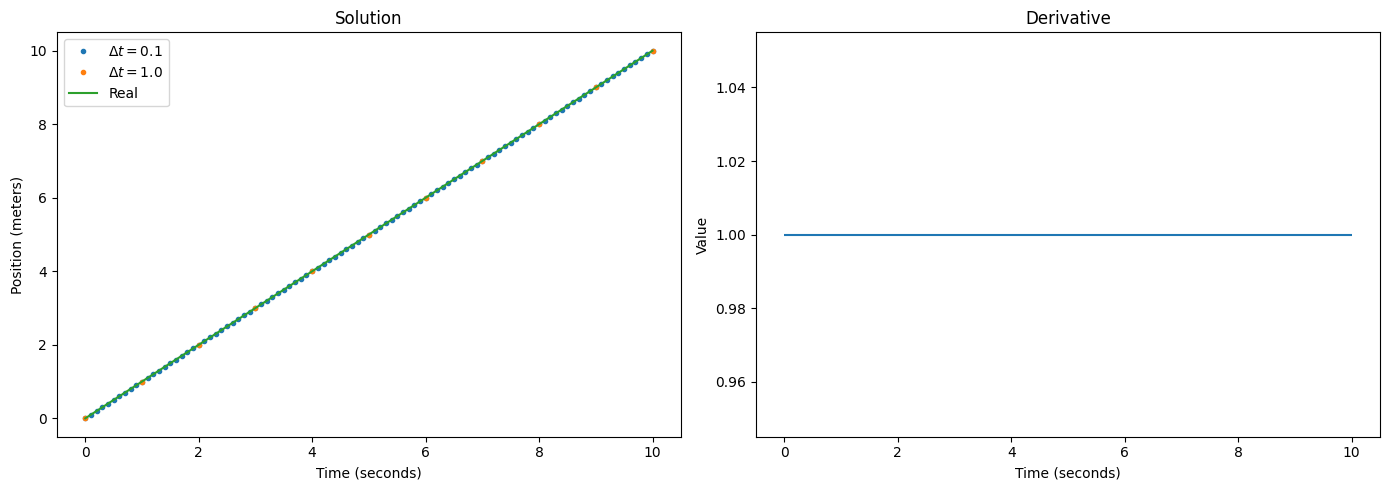
Case 1: Constant Speed
Say our rocket engine, once started, instantly accelerates our car to a speed of 1, and it stays at that speed forever. Thus, $\frac{dx}{dt} = 1$ for all $t$. The solution is simply $x(t) = t$, i.e. after $t$ seconds our car will have travelled $t$ meters. We could also get an exact solution via Euler’s method sketched in the previous section. In fact, it doesn’t even matter how large the discretization step $\Delta t$ is – we can instantly jump to any desired $t$ simply by following the derivative, without knowing the functional form of $x(t)$.
Case 2: Burst of Speed
To have something slightly more interesting, say the rocket instantly accelerates the car to a speed of 1, but then fizzles out, leading to the car slowing down due to factors like friction and air resistance. Let’s set $\frac{dx}{dt} = \frac{1}{t + 1}$.1 Solving this integral requires a slightly better grasp on calculus, but is still easy: $x(t) = \log(t + 1)$. The car will slow down to a crawl over time, but it will actually never stop, since the logarithm keeps growing forever.
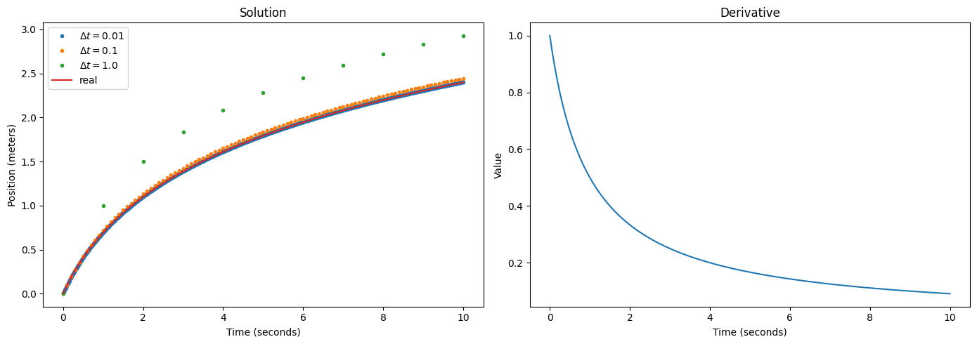
We can once again try Euler’s method. This time, we can see the influence of $\Delta t$: The larger it is, the more we deviate from the true solution. In fact, we require around one hundred steps per second to achieve a good fit. Unfortunately, Euler’s method is not very usable in practice: $\frac{dx}{dt}$ may be expensive to evaluate, in which case the number of steps required makes it prohibitively slow. Let’s look another example, along with a better approximation method:
Case 3: Wind Tunnel
The two examples above are not “real” differential equations in that the derivative is not dependent on the function itself. We just computed some integrals. Let’s build upon Case 2, but say the car is in a wind tunnel, with a current blowing against it that becomes stronger as it moves forward. A very simple model could be $\frac{dx}{dt} = \frac{1}{t + 1} - \frac{x}{10}$. This means the wind becomes stronger in a linear fashion as the car moves forward, and as the rocket boost becomes weaker, it will eventually push the car back.2
This problem has suddenly become much more difficult. We need a function $x(t)$ such that its derivative is the negative of itself divided by 10, plus $\frac{1}{t+1}$. Solving such a differential equation requires special methods that go beyond the point of this article. But this can be solved (e.g. using Wolfram Alpha) to be
\[x(t) = \left(\frac{\mathrm{Ei}\left(\frac{t+1}{10}\right)} {\exp\left(\frac{1}{10}\right)} + c\right) \exp\left(-\frac{t}{10}\right)\]where $\mathrm{Ei}$ is the exponential integral.3 Below, we once again show a curve of the solution along with Euler’s method for various $\Delta t$. This time, we also showcase a second-order Heun solver.
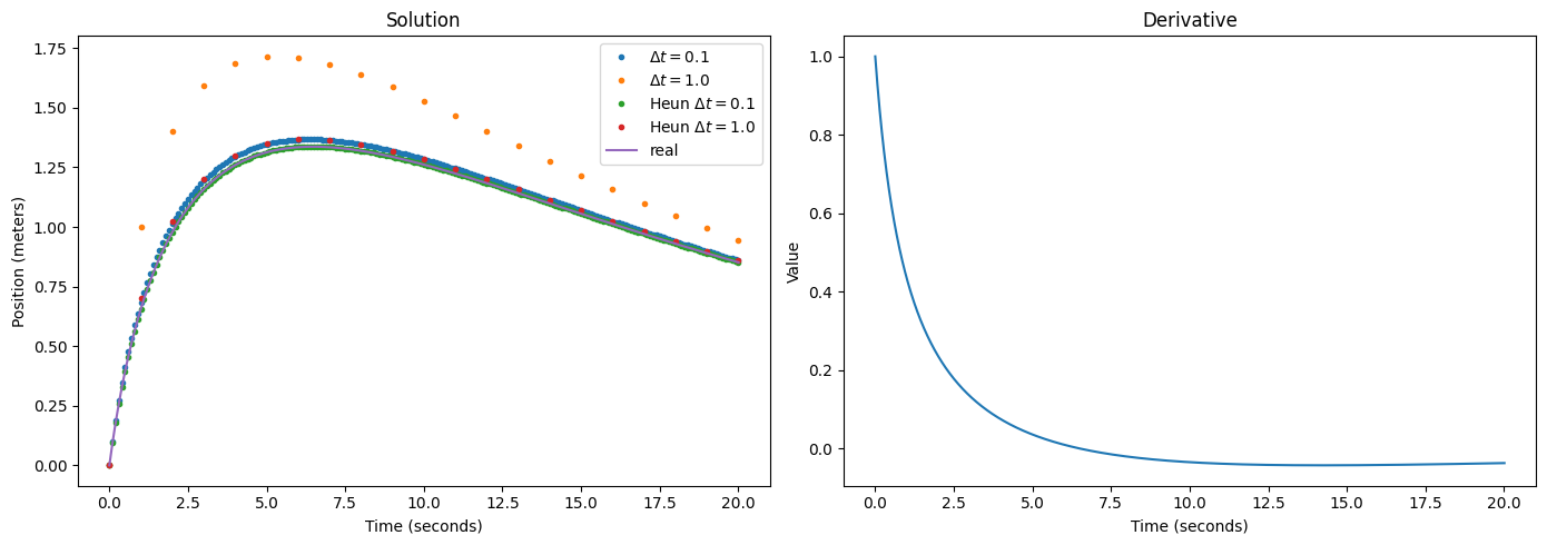
We can see that the second-order method with $\Delta t = 1$ matches the first-order solution with $\Delta t = 0.1$. Since the second-order method requires two evaluations per step, this implies a 5x speedup for a similar solution quality! Going down to $\Delta t = 0.1$ with a second-order method gives a very good match with the true solution, save for slight deviations at the start.
There are higher than second-order solvers, as well. You can read up on the general family of Runge-Kutta methods, if you wish. However, we will now consider what happens when you add a random component to a differential equation.
Stochastic Differential Equations
The differential equations we have considered so far are fully deterministic. However, as we have discussed previously, many real-world processes are so complex to model as to be essentially random. For example, consider our rocket car in the wind tunnel: It’s unlikely that the force of the wind is perfectly consistent. Rather, the turbulent movement likely induces a somewhat “random” force at each point in time and space. Aside from that, stochasticity also plays an important part in generative models. As such, it may be useful to have some sort of stochastic analogue of ordinary differential equations. We will not treat this in any theoretical detail, but the major results here come from Itô calculus. As a stochastic differential equation (SDE), we can understand an equation of the form:
\[dx = f(x, t)dt + g(t)dw\]Here, $f(x, t)$ is called the drift, and $g(t)$ the diffusion coefficient. $dw$ is the so-called Wiener process. This is essentially infinitesimal Gaussian noise. Crucially, when you discretize the SDE and take a step of size $\Delta t$, this will add Gaussian noise with mean 0 and variance $\Delta t$.
To illustrate what an SDE might look like, say we update our wind tunnel example as follows:
\[dx = \left(\frac{1}{t + 1} - \frac{x}{10}\right)dt + \sigma dw\]Here, $f(x, t)$ is as before, and $g(t)$ is a constant. Clearly, we cannot “solve” this SDE in a classical sense, as due to the random component, there is no longer any fixed value $x(t)$. Rather, we would now have to consider probability distributions $p_t(x)$. That is, given some initial value $x_0 = x(0)$, for each $t$ we have a distribution $p_t(x \mid x_0)$, which gives the probability that the initial value $x_0$ is mapped to a specific value at time $t$. But the value at $t=0$ could also be random, $x_0 \sim p_0(x)$.
However, we will not concern ourselves with how to solve SDEs, i.e. how to find $p_t$. Discretization is still easy, albeit non-deterministic. Here are examples of several runs of the above SDE at $\Delta t = 0.01$ with different choices for $\sigma$. For each choice, we do 100 runs, each of which is represented by one line.
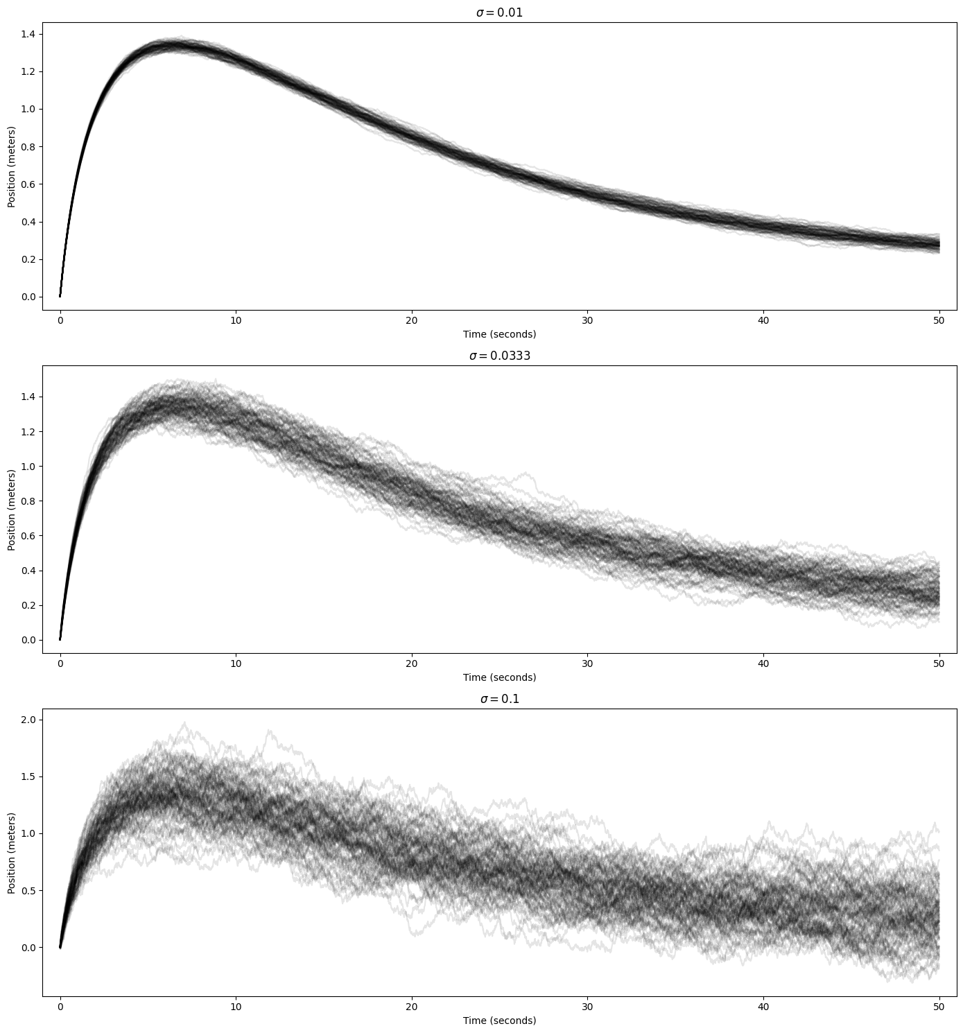
The results are as can be expected: For small noise levels, the runs are fairly consistent. The larger the noise, the more chaotic it becomes. Interestingly, the randomness seems worse later in the run, with early values being relatively more consistent. There are likely two reasons for this:
- Specific to our SDE, $f(x, t)$ tends to be larger at the start, meaning it is more impactful compared to the constant diffusion coefficient. At later steps, the drift becomes weaker, meaning that the random component has a stronger influence on the movement.
- In general, the random deviations accumulate over time and push $x(t)$ “off course” to different positions, which will lead to each run experiencing different drift values, and this in turn changes the trajectory of each run on top of the random noise component.
We will leave it at this high-level look at SDEs in general. Rather, we now turn to how they can be used for generative modeling.
From Score Matching to SDEs
Note: This section heavily relies on the original paper by Yang Song et al.
Recall (or see the papers if you need a refresher) that both score-based and diffusion generative models work by learning to reverse a “diffusion process” that turns data into noise. Since this process is somewhat simpler for classic score-based models, we will consider those first. We define a sequence of geometrically increasing noise levels $\sigma_t,\ t=1, \ldots, T$. Then, given some data $x_0$, we have $x_t = x_0 + \sigma_t\epsilon$, where $\epsilon \sim \mathcal{N}(0, 1)$ is a standard Gaussian sample. This way, we can get a sequence of $x_t,\ t=1,\ldots\,T$, and clearly, $p(x_t \mid x_0) = \mathcal{N}(\mu = x_0, \sigma^2 = \sigma_t^2)$, i.e. $x_t$ is a Gaussian around $x_0$, and with the corresponding variance.
However, each $x_t$ is just defined in terms of the original $x_0$. While this is practical, as we can just jump directly to any desired $t$, this does not build a good connection to SDEs, as these are defined in the change in $x$ from one step to the next. However, we can write an equivalent formulation as $x_t = x_{t-1} + \sqrt{\sigma_t^2 - \sigma_{t-1}^2}\epsilon$.4 Note that this is a Markov chain – each sample only depends on the previous one! Another way of writing this is $\Delta x = x_t - x_{t-1} = \sqrt{\sigma_t^2 - \sigma_{t-1}^2}\epsilon$. This gives the change between successive values $x_t$.
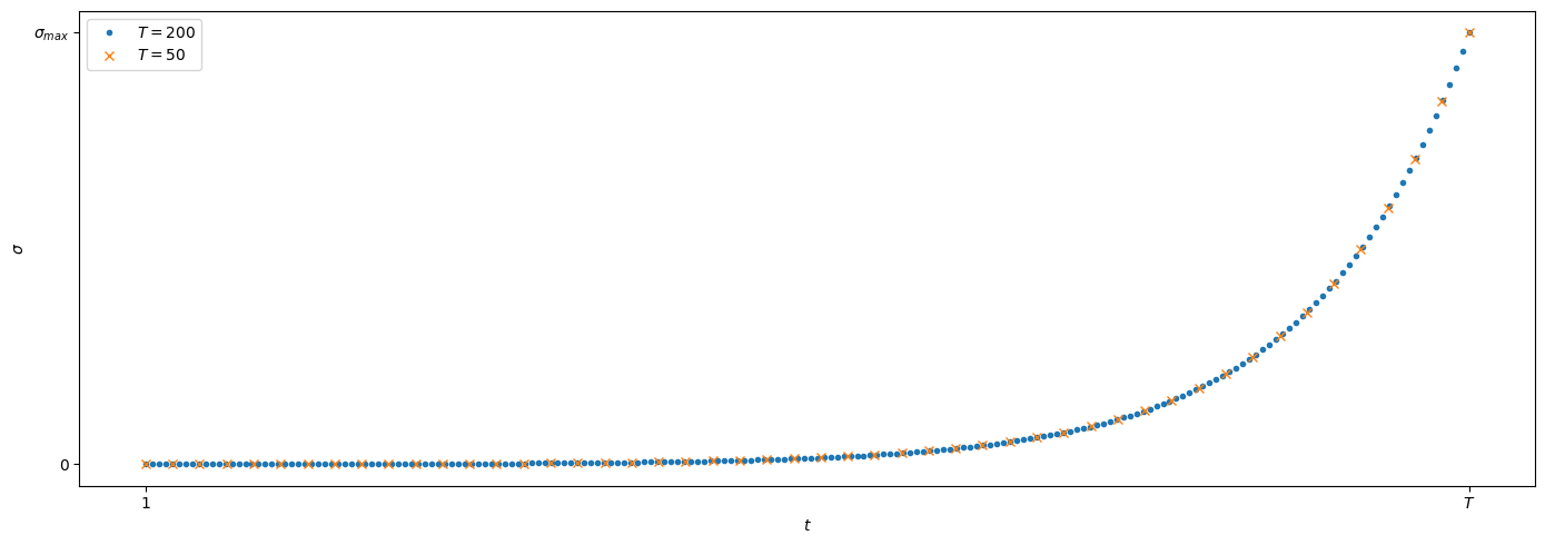
Now, for score-based models, we usually define $\sigma_1 = \sigma_{min}$ to be a very small value, such as 0.01 for images in range [0, 1], and some $\sigma_{T} = \sigma_{max}$ that is large enough to “drown the data in noise”. These values are fixed independent of how large $T$ is. Thus, if we increase the number of noise levels $T$, successive levels have to move closer together, as illustrated below:
Let’s make a small change to the notation. The indices we have chosen are clearly arbitrary. We could just redefine $\sigma_T \rightarrow \sigma(1)$, and $\sigma_t \rightarrow \sigma\left(\frac{t}{T}\right)$. All we did was fix $T \rightarrow 1$, and “squeeze” the other indices into the range [0, 1], accordingly. We also changed notation from indices to function values. But mathematically, nothing has changed! However, this prepares us for the next step.
Now imagine what happens if we were to increase $T$ to infinity, that is, if we kept adding more noise levels to the point that we have infinitely many. Because $\sigma_{min}$ and $\sigma_{max}$ remain fixed, the infinitely many noise levels have to squeeze into a fixed-size space, meaning that successive noise levels have to be infinitely close together. At this point, we have moved from discrete noise levels to a continuous space, with $t$ taken from a “time” interval [0, 1].5 Now:
- $x$ and $\sigma$ become functions of $t$ instead of discrete sequences.
- The difference between successive values of $x$, $\Delta x$, becomes a derivative $dx$.
- The difference between successive values of $\sigma^2$ also becomes a derivative: $\sqrt{\sigma_t^2 - \sigma_{t-1}^2} \rightarrow \sqrt{\frac{d\sigma^2(t)}{dt}}$
- The standard Gaussian noise $\epsilon$ becomes infinitesimally small – a Wiener process $dw$.
Thus, we have arrived at an SDE:
\[dx = \sqrt{\frac{d\sigma^2(t)}{dt}}dw\]Here, $g(t) = \sqrt{\frac{d\sigma^2(t)}{dt}}$ and $f(x, t) = 0$.
For $\sigma(t)$, we can choose the following exponential function to mirror the usual geometrically increasing sequence:
\[\sigma(t) = \sigma_{min}\left(\frac{\sigma_{max}}{\sigma_{min}}\right)^t\]And then we can solve:
\[\sqrt{\frac{d\sigma^2(t)}{dt}} = \sigma_{min}\left(\frac{\sigma_{max}}{\sigma_{min}}\right)^t \sqrt{2\log\frac{\sigma_{max}}{\sigma_{min}}}\]which we can use as a concrete choice for $g(t)$. Because this process leads to a continuously growing variance, this is called the variance exploding or VE SDE. Finally, we have arrived at an SDE that we can use to turn our data into noise. In fact, you can show that $p_t(x \mid x_0) = \mathcal{N}(x_0, \sigma^2(t))$, so this is an exact analogue to the original discrete process. But what about a generative model?
Sampling via the Reverse SDE
It turns out, for the general SDE formulation of $dx = f(x, t)dt + g(t)dw$, a reverse can be found with relative ease:
\[dx = \left[f(x, t) - g(t)^2 \nabla_x \log p_t(x)\right]dt + g(t)dw\]Here, $dt$ is a negative time step. Crucially, this reverse SDE contains the score $\nabla_x \log p_t(x)$. The other components are already known from the forward SDE. This gives us a basic recipe for training and sampling a score model based on SDEs:
- Training (for each step):
- Sample $t \in [0, 1]$.
- Given data $x_0$, sample $x_t \sim p_t(x \mid x_0)$.
- Perform a standard score matching training step using $x_0$, $x_t$, and our model.
- Sampling:
- Start with a random sample $x_1 \sim \mathcal{N}(0, \sigma_{max}^2)$, which approximates $p_1(x)$.
- Run the reverse SDE using the trained score model and a solver of your choice.
The second point for training corresponds to running the forward SDE up to time $t$, but for most practical cases you can actually compute $p_t$ directly, without iteration, which makes training very efficient, just as with standard score-based or diffusion models.
The SDE perspective opens up various paths for improving on “standard” denoising score matching models. Due to the length of this article, we only briefly discuss a couple here.
Diffusion Models as SDEs
Although they look somewhat different on the surface, DDPMs can be expressed in the exact same format. Here we have the diffusion process $x_t = \sqrt{1 - \beta_t} x_{t-1} + \sqrt{\beta_t} \epsilon$. Again, $x_0$ is the original data, and this process always converges to a standard normal distribution, as long as the noise schedule $\beta_t$ is chosen appropriately. If we decide to use “infinitely many” noise levels, where each step becomes infinitely small, we again end up with a continuous process, namely $dx = -\frac{1}{2}\beta(t)xdt + \sqrt{\beta(t)}dw$. Thus, we have an SDE with drift $f(x, t) = -\frac{1}{2}\beta(t)x$ and diffusion $g(t) = \sqrt{\beta(t)}$, which is called the variance preserving or VP SDE.
In fact, you can show that diffusion models perform score matching even without the SDE connection. This can be exposed by rewriting the respective training algorithms somewhat, meaning that these models are already trained to output scores for noisy data. This, in turn, means we can use them for sampling via the reverse SDE.
New Model Types
Different choices for $f(x,t)$ and $g(t)$ can lead to new models. Of course, not all choices for these functions will make sense. However, the paper showcases one new SDE that is inspired by diffusion models, but adds noise less slowly, termed the subVP SDE, which tends to perform very well.
New Sampling Algorithms
Since we generally cannot solve these complex reverse SDEs in closed form, we have to employ discrete sampling methods. As previously discussed, the most basic method for ODEs is the Euler method. There is an analogue for SDEs called Euler-Maruyama. This is basically the Euler method, but incorporating random normal noise from the discretization of the Wiener process. This method is extremely general, and can easily be applied to any discretization of any SDE. In fact, it’s what we used for the “turbulent wind tunnel” example further above.
However, we can also make use of our knowledge of the original discrete process. For example, recall that for discrete score-based models, $x_t = x_{t-1} + \sqrt{\sigma_t^2 - \sigma_{t-1}^2}\epsilon$. This means we can construct a discrete analogue of the diffusion coefficient $g(t)$:
\[G_t = \sqrt{\sigma_t^2 - \sigma_{t-1}^2}\]Then, we can sample down from $x_T$ to $x_0$ in $T$ discrete steps. This differs from Euler-Maruyama in that we can use our knowledge of the current and next noise levels in the discrete chain, rather than just the instantaneous change in noise level, which is given by $g(t)$. We are basically constructing a “classic” score-based model after training on a continuous range of noise levels. This also means that we can choose the number of noise levels $T$ freely. The same procedure can be done for the VP SDE, restoring “classic” diffusion models, or the subVP SDE, as well.
The above is termed the reverse diffusion sampler in the paper. Other samplers discussed there include:
- Ancestral sampling as used for the original diffusion models, with a derivation included for score-based models, as well.
- Corrector samplers, which correspond to annealed Langevin dynamics, the sampling method originally used for score-based models.
- Predictor-corrector samplers, which combine an SDE discretization like reverse diffusion with corrector methods by using them alternatingly.
Finally, they also connect back to ordinary differential equations (ODEs). Remember that those are deterministic! The remainder of this article will focus on the ODE perspective, which has become very popular in recent years.
ODEs for Generative Modeling
Remember the forward SDE turning data into noise:
\[dx = f(x, t)dt + g(t)dw\]As it turns out, you can construct an ODE that has the same marginals. That is, given the data distribution $p_0(x)$, the diffused distribution $p_t(x)$ will be the same for any specific $t$, no matter if we use the SDE or the equivalent ODE. This means that if the SDE maps a data distribution to, say, a standard normal distribution, the equivalent ODE will do the same when considering the data distribution as a whole. Of course each individual sample will be treated differently, as the equations are different. This ODE is called the probability flow ODE and is given by
\[dx = \left[f(x,t) - \frac{1}{2} g(t)^2 \nabla_x\log p_t(x)\right] dt\]Note that this is the forward ODE turning data into noise; but an ODE is very easy to reverse by simply running time backwards. Thus, the reverse ODE is the exact same equation, but with negative $dt$. Compared to the reverse SDE given earlier, the Wiener process $dw$ has disappeared, and $g(t)$ has acquired a factor of $\frac{1}{2}$. Because this is a completely deterministic equation, if we start generating from a specific random noise point at $p_1$, we will always generate the same data point. This contrasts with SDEs, where the random component at each step will lead to different generations when starting from the same noise sample multiple times. Furthermore:
- The forward ODE is deterministic, meaning a data point from $p_0$ will always be mapped to the same noise point in $p_1$.
- Forward and backward equations are inverses of each other, meaning we can “encode-decode” data samples to noise and back again. Save for discretization error, the ODE is invertible!
- $p_1$ can act as a proper latent distribution, allowing for applications such as interpolating between samples.
Intuition on Stochastic vs Deterministic Transformations
At this point, you may wonder how it can even be possible that an SDE and an ODE can transform a given data distribution to the same noise distribution. We will illustrate this with a simple example.
Consider the task of transforming a standard normal distribution $p_0$ to a normal distribution $p_1$ with mean $\mu_1 = 0$ and variance $\sigma_1^2 = 4$. Formally, we are given $x_0 \sim \mathcal{N}(0, 1)$, and want to find a transformation $f$ such that $x_1 = f(x_0) \sim \mathcal{N}(0, 4)$. Let’s consider two options.
Option 1: Adding another random variable
The sum of two normal random variables also follows a normal distribution. The means and variances simply add up. We could define an auxilliary variable $x_a \sim \mathcal{N}(0, 3)$ and set $x_1 = x_0 + x_a$. Then, $\mu_1 = \mu_0 + \mu_a = 0$, and $\sigma_1^2 = \sigma_0^2 + \sigma_a^2 = 1 + 3 = 4$ as desired.
Option 2: Multiply by a constant
When a random variable is multiplied by a constant number, the variance is multiplied by the square of that constant, and the mean is multiplied by the constant. This means we can set $x_1 = 2x_0$. Then, $\sigma_1^2 = 2^2 \sigma_0^2 = 4$. Also, the mean $\mu_1 = 2\mu_0 = 0$.
It seems like both options work: $x_1$ has the desired distribution in either case. However, the methods differ significantly. The first option is stochastic: If we were to take the same sample $x_0$ and transform it to $x_1$ twice, we would most likely get different results, since a different random value $x_a$ is added each time. In contrast, the second option transforms any given sample in th exact same way each time. This trivially implies that both methods will lead to different results when applied to a specific sample. And yet, when considering the distributions $p_0$ and $p_1$, both methods are the same! This shows that stochastic and deterministic transformations can be equivalent when considering distributions as a whole.
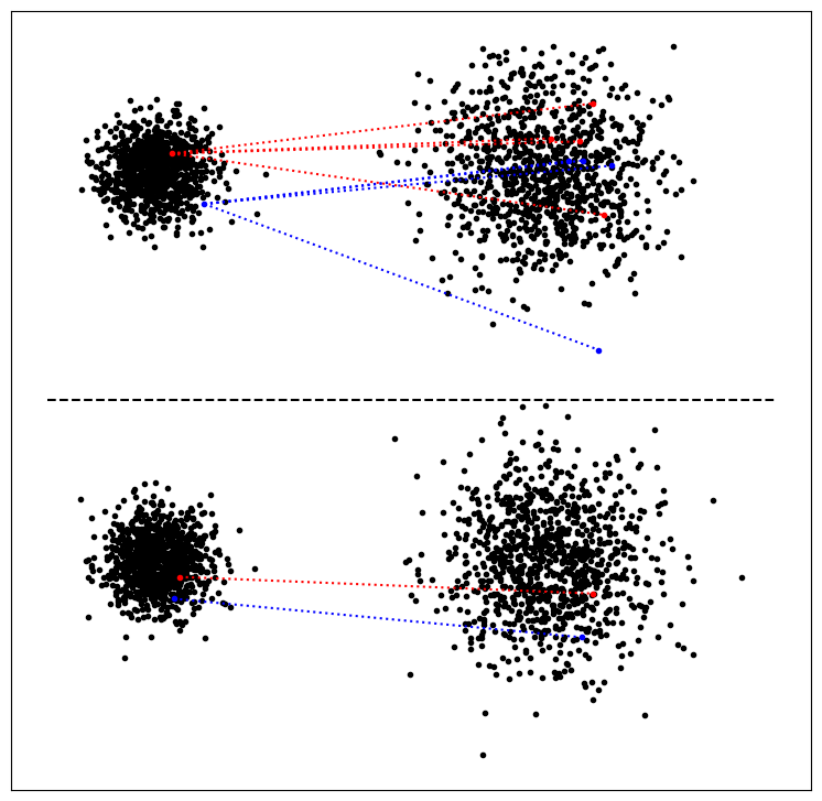
Below, you can see a graphic comparing both options empirically. On the left is $p_0$, on the right $p_1$. Top is the stochastic transform, bottom the deterministic one. For each, we also highlighted some specific points. For the stochastic one, we transform each “source” point multiple times, and we can see how the results differ. There is a vague relation between original and transformed points – the red point is originally somewhat higher up, and the transformations tend to be higher, as well. But this is not guaranteed. In contrast, for the deterministic transformation, the shape of the distribution is preserved exactly, as are relations between the different samples. However, the overall distributions look similar between the two cases.
Other Differential Equation Formulations
To close out this article, we will look at some more recent advancements in the field.
Modern Diffusion Models
First off, you may come across slightly different SDE/ODE formulations than the one we have seen so far. An influential paper by Tero Karras et al. formulates SDEs directly in terms of the $p_t$ they induce. Recall that we start with a data distribution $p_0$, and data $x_0$ is transformed (“diffused”) by the forward SDE to $x_t \sim p_t(x \mid x_0)$. However, the form of $p_t$ has to be inferred from the drift and diffusion coefficients, $f(x, t)$ and $g(t)$.
The authors propose to completely remove these coefficients, and instead work directly with an input scaling $s(t)$ and a noise schedule $\sigma(t)$, such that $p_t(x \mid x_0) = \mathcal{N}\left(s(t)x_0, \sigma^2(t)\right)$. This allows us to see directly how the input is scaled and how much noise is added at each time $t$, which should also make it easier to design new schedules. The authors then rewrite the actual ODE/SDE used for sampling in terms of the functions $s(t)$ and $\sigma(t)$. See the paper for details. In particular, equation 81 gives the full ODE.
Flow Matching
The above formulation still leads to a somewhat restricted class of functions. Even if you set $s(t) = 1$, corresponding to the VE SDE (as they do in the paper), you get
\[dx = - \dot{\sigma}(t)\sigma(t) \nabla_x \log p_t(x) dt\]where $\dot{\sigma}$ denotes the derivative of $\sigma$. This means that the ODE has to involve the product between a function and its own derivative.
The authors of the Flow Matching technique instead propose to think directly in term of probability paths, which is just the collection of the diffused distributions $p_t$ for all $t$. That is, we ask “what is the path we want to take from $p_t$ to $p_{t’}$?” Unfortunately, the terminology and notation in the paper is quite different from what we have considered so far, making it somewhat difficult to understand. But they connect back to flow models, specifically continuous normalizing flows. In what follows, we will be adapting some of the notation to be more similar with the rest of this article.
Basic Description
Recall that in flows, we want to transform a simple distribution $p_0$ into the data distribution $p_1$ (unfortunately, this is reversed from the SDE literature) via a series of invertible transformations. These transformations often only make a small change to the input. Consider what would happen if we added more and more layers to the flow. Since $p_0$ and $p_1$ are fixed, each layer would have to make a smaller and smaller change. In the limit, you have infinitely many layers making infinitely small changes – a continuous process! Since flows compute deterministic functions, this is an ODE:
\[dx = v_t(x)dt\]That’s it! You can imagine $v_t$ being a neural network that directly outputs the change in $x$ (“velocity”), rather than a score function. Integrating this velocity over $t$ then defines a flow $\psi_t(x)$. Instead of having many “flow layers”, we have one function that is dependent on $t$ (the “depth” of the layer). The ODE form also means this flow is trivially invertible (save for discretization error).
$v_t(x)$ can be understood to mean the same as $v(x, t)$. Flows are trained by mapping the data back to the simple distribution $p_0$, and maximizing the probability there. Unfortunately, this requires running the full ODE for each training step, which is very slow. Flow Matching improves this by deriving a training recipe that works at single time steps. We will not discuss details here, but at a high level, this is it:
- Define a conditional flow $\psi_t(x_0 \mid x_1)$ that determines how a noise sample $x_0$ is transformed to a data sample $x_1$.
- Figure out the correct conditional vector field $u_t(x \mid x_1)$ such that $d\psi_t(x_0 \mid x_1) = u_t(\psi(x_0 \mid x_1) \mid x_1)dt$, i.e. $u$ is the derivative of $\psi$. 6 By construction of the flow, $u$ will point towards $x_1$.
- Train the neural network $v_t(x)$ to match $u_t(x \mid x_1)$ along the entire trajectory of $t$, for noisy inputs $x \sim p_t(x \mid x_1)$.
- $p_t(x \mid x_1)$ can be sampled by sampling random $x_0 \sim \mathcal{N}(0, 1)$ and applying $\psi_t(x_0 \mid x_1)$.
Roughly speaking, the network has to figure out the direction towards the clean data $x_1$ from the noisy input $x \sim p_t(x \mid x_1)$. After training succeeds, we can then take a random sample from $p_0$ and follow the direction given by the neural network output. In practice, we are discretizing an ODE!
Intermezzo: Conditional Probability Paths & Score Matching
The fact that we are using conditional flows and vector fields is crucial for Flow Matching to work in practice. Let’s think back to score matching models. The goal is to learn the score $\nabla_x \log p_t(x)$ for the noisy distributions $p_t$. However, we don’t actually have access to these distributions, as they depend on the unknown data distribution $p_0$. Instead, we only ever work with the conditional distributions $p_t(x \mid x_0)$, i.e. putting noise onto specific data samples $x_0$. For these distributions, we can easily know the functional form (e.g. a Gaussian centered around the data point), which gives us a properly defined target for training.
The “magic” of denoising score matching is that matching the conditional scores also leads to the model learning the marginal scores in expectation, but this is not trivial! The same can be derived for Flow Matching, which is likely also where the name comes from: Matching the conditional vector fields of the conditional flows will also lead to matching the marginal vector field corresponding to the desired probability path.
Flow Matching in Practice
The given ODE format allows for more flexibility in the choice of probability paths. The authors consider a general form of affine flows:
\[\psi_t(x_0 \mid x_1) = \sigma_t(x_1)x_0 + \mu_t(x_1)\]If $x_0$ is initially drawn from $\mathcal{N}(0, 1)$, this results in a distribution $p_t(x | x_1) = \mathcal{N}(\mu_t(x_1), \sigma_t^2(x_1))$. As long as $\mu_1(x_1) \approx x_1$ and $\sigma_1(x_1) \approx 0$, the flow will always “end” in the data $x_1$.
Specifically, the authors propose to use a flow that simply computes a linear interpolation between noise and data:
\[\psi_t(x_0 \mid x_1) = (1 - t)x_0 + tx_1\]Then, $u$ evaluated at the flow output is just the derivative with respect to $t$:
\[u_t(\psi_t(x_0 \mid x_1) \mid x_1) = x_1 - x_0\]This is simply the difference vector between original data and random noise, and it’s the same for all $t$! The network $v_t$ will receive the partially noisy input $\psi_t(x_0 \mid x_1)$, and try to match the target velocity $u_t$.
This setup is ideal in the sense of optimal transport (OT). Roughly, this leads to the path between noise and data being perfectly straight, and move at a constant speed. However, this only holds for the conditional flow given a real data sample $x_1$, and not necessarily for the actual sampling trajectory starting from pure noise. The framework also allows for different paths: For example, ODEs corresponding to the VE/VP/subVP SDEs considered previously can also be derived. Still, the main attraction is the OT path, which is supposed to lead to faster and more stable training, and allow for sampling with fewer steps. This makes sense: The more linear (“straight”) the path, the less discretization error we obtain with a given number of steps. A perfectly straight path could be sampled with no error via a single Euler step.
Other Recent Models
Finally, we mention related frameworks for constructing generative models with ODEs. Rectified Flows are extremely similar to Flow Matching. They also introduce the idea of reflow, where you train multiple models in sequence, which are supposed to successively straighten the probability paths, to the point that you can eventually get respectable results via a single sampling step, jumping directly from $x_0$ to $x_1$.
Consistency Models are trained to produce the same output from any point along the ODE path, with the output for the data $x_0$ (yes, we are switching again…) being forced to be $x_0$ itself. This eventually results in the model learning to output clean data $x_0$, no matter the noise level of the input. In the best case, this can also allow for single-step sampling.
Conclusion
We can actually tie back the discussion to the initial “rocket car” example, but now the situation is a little different. You want to go from $a$ to $b$, and have to build the best engine to get there reliably. Initial attempts were mostly concerned with getting there at all. No we are entering the phase where it’s all about getting there quickly and reliably, and stopping at the appropriate place. What kind of engine seems to be the best: One that starts quickly, then slows to a crawl? One that speeds up in an exponential fashion? Or one that just moves at a constant speed? You decide. ;)
Using differential equations for generative modeling is a very active and complex field. This article only gave a brief look at the basics and some current models. The unfortunate reality is that this field is mathematically challenging, fast-moving, and uses inconsistent terminology. As such, really getting into it requires a lot of work. We hope that you could at least obtain a basic understanding of the concepts involved. A deep appreciation of the finer details will require sitting down and implementing and tinkering with these models yourself. Have fun!
-
Please note that I’m not a physicist, in fact I’m terrible at physics, and all these examples are just made up numbers/functions with no relation to reality. ↩
-
In fact, it will push the car forward if $x < 0$. See footnote 1. ↩
-
The current version of Wolfram Alpha seems to give a different form of the solution. ↩
-
In case you want to prove that this gives the same $p(x_t \mid x_0)$, keep in mind that when we add two or more independent random variables, their variances add together. ↩
-
Note that the choice of this interval is completely arbitrary; it is simply mathematically convenient. Any other interval could be used with some care. ↩
-
This statement is technically somewhat imprecise. The derivative of $\psi_t(x)$ is not $u_t(x)$ – it’s $u_t(\psi_t(x))$. This is why the $u$ functions given in the paper for specific probability path look more complex than they might need to be – they are given as $u_t(x)$, but we generally use the form $u_t(\psi_t(x))$. ↩