Investigating Compression with VQ-VAEs

A while ago, I was experimenting with Residual Vector-Quantized Variational Autoencoders (RVQ-VAE) for the application of latent diffusion for music generation. However, I was never quite happy with the reconstruction quality that I got. This prompted me to investigate RVQ-VAEs in a simpler image reconstruction task, investigating the effect of varying codebook size, number of codebooks, and latent space size on reconstruction performance. I found some quite interesting regularities which I would like to discuss in this post.

VQ-VAE Basics

VQ-VAEs were introduced in 2017 for discrete representation learning. In a standard autoencoder, data points are mapped to arbitrary latent representations. In variational autoencoders, each data point is mapped to a probability distribution instead. Usually, continuous distributions are chosen, with the most common choice being Gaussians. VQ-VAEs, on the other hand, encode data to discrete representations. To achieve this, first a regular autoencoder is applied. Next, each latent vector is mapped to the closest vector in a codebook, which is also part of the model, and learned alongside the other parameters. This means that the latent representations are limited to combinations of the codebook vectors. For more details, please read the paper linked above.
The discrete latent space has some unique advantages over regular VAEs. For example, we can compress high-dimensional data to a smaller discrete representation, and then train an autoregressive model to generate such representations, which can then be decoded back into the original space. Such techniques are used in models like MusicGen to generate music with high sampling rates relatively efficiently.

Compression With Autoencoders

VQ-VAEs have a major advantage over regular autoencoders in terms of the compression they can achieve in the latent space. As an example, let’s say we are working with color images of size 256x256. Perhaps we train a convolutional autoencoder to compress these to a size of 32x32. On the surface, this seems like a reduction by a factor of 64, since that’s the reduction in the number of pixels. However, we generally have a larger number of channels in our latent representation! Color image have three channels, but our encoding may have a lot more. Let’s say we have 256 channels in the latent space. This is more than 80 times more than the input, completely negating the reduction in pixels! Additionally, we usually encode to floats, which are often stored at 32bit precision, whereas images are often only stored in 8bit precision. This means our autoencoder blows up the representation by another factor of 4! Overall, our “compressed” latent representation takes more space than the original images. Of course, we could play around with the parameters to alleviate this, but we will have a hard time achieving strong compression while retaining good reconstruction quality.

This is where VQ-VAEs shine: Since we have a limited number of codebook vectors, and we know that each “pixel” in the encoding is one of those vectors, we do not actually need to store the full encodings. Rather, we only need to store, for each pixel, the index of the codebook vector at this point. The codebook, meanwhile, needs to be stored only a single time, no matter how many images we encode. The number of bits per codebook index depends on the size of the codebook. For example, a codebook with 1024 entries would require indices from 0 to 1023, which require 10 bits to store. Thus, in this example, each pixel would only require 10 bits to store the index, down from 32*256 in the example above (32 bits per float times 256 channels). Finally, we can actually achieve proper compression!

Exploring Compression

When training autoencoders, there are many moving parts: Dataset, architecture, latent space structure, reconstruction loss… I conducted some experiments where I tried to simplify things as much as possible. I trained a convolutional autoencoder to minimize mean squared reconstruction error on CIFAR10. The architecture is fixed, except for the number of channels d in the final encoder layer, which are varied systematically. As such, images are encoded to 4x4xd, down from the 32x32x3 input size. The results can be seen below.

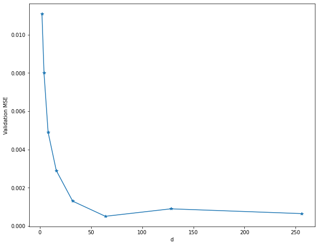
Unsurprisingly, more channels, i.e. a larger latent space, results in better reconstructions, as the model can simply store more information in a larger space. I’m not sure why performance slightly degraded when using d=128; there may have been some instability in the training as the model starts to overfit. Subjectively, a loss of around 0.002-0.003 is where the reconstructions start looking “acceptable”, so in this case, d=16 is a kind of lower bound for acceptable performance. Of course, a different (e.g. larger) architecture may be able to compress more efficiently, and thus manage with a smaller d. On the other hand, performance plateaus after d=64. My goal here was not to find the best possible architecture; rather, this just serves to provide a baseline performance for the following VQ-VAEs.

Introducing VQ

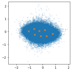
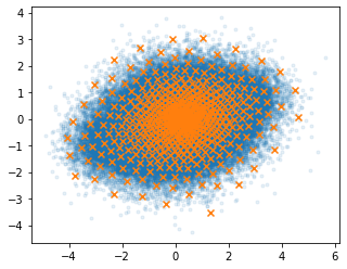
When using VQ-VAEs, we introduce another main variable: Codebook size k. That is, in addition to d, how many vectors do we allow in the codebook? Obviously, more vectors can cover the latent space more densely, which should be beneficial for reconstruction performance, as the quantization becomes more precise. Compare the two figures below; each orange cross is one codebook vector. The first only uses 8 codebook vectors, the second one uses 512.

However, more vectors also means less compression. As such, we only want to use as many vectors as actually necessary. Here are the results; this time, each d is represented by a different line, whereas the new parameter k is on the x-axis.

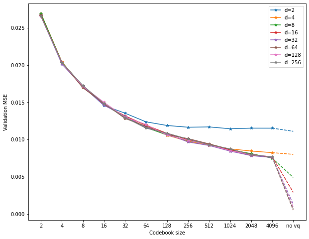
Things look quite a bit different this time: While performance still improves with larger d as well as k, there is an interaction between the two. To be precise, codebook size k seems to put a hard limit on the benefits of larger d. In fact, even with a rather large 4096 codebook entries, performance maxes out at d=8, with no benefits for more latent channels. Also, already for d=8, performance lags far behind the basic no-VQ autoencoder. It seems an absurd number of codebook entries would be required to catch up.

These observations make sense: For larger d, the overall size of the space increases exponentially. As such, we require many more codebook entries to properly “fill out” the space. Thus, we quickly arrive at a situation where the model cannot make use of the larger d, as the codebook vectors simply cannot make use of the available space.

This obviously presents us with a bit of a problem. If VQ-VAEs result in unacceptable reconstruction performance, their compression advantage is not useful. Recall that I mentioned a loss of around 0.002-0.003 is a good minimal target for this task. None of the VQ models even come close to this value, in fact barely reaching around 0.007 or so. Increasing the codebook size becomes infeasible at some point.

We can understand this mathematically. Recall that, for k=1024, each “pixel” in the encoded image requires 10 bits to store the codebook index. This is the “bit depth” of each sample. Also, in our architecture, we encode each image to a 4x4 array of indices. That is, there are 16 vectors per image. This puts us at 16*10=160 bits per image. Compare this to the original: 32x32 pixels, 3 color channels, 8 bits per value. This puts us at 32*32*3*8 = 24576 bits per image. We are compressing by a factor of 153.6. What if we are okay with more bits, i.e. less compression? We can either increase the number of vectors, that is, compressed image size (say, to 8x8), or the bit depth. Increasing the image size can have negative consequences for downstream applications. For example, if we wanted to train a generative model on the latent space, we only need to generate 16 vectors for a 4x4 image, whereas we would need 64 vectors for an 8x8 image, meaning four times more effort. The other option is to increase bit depth, which is drectly related to codebook size k. Maybe we are okay with 2x less compression, i.e. increasing bit depth from 10 to 20. But 20 bits correspond to 2**20 codebook entries – over a million! This is infeasible, and hints to why increasing k is not effective: Each doubling of codebook size adds only a single bit of information per vector. Clearly, we need some other method to increase the capacity of our codebooks.

Residual VQ

The basic idea of residual VQ (RVQ) is to use a series of codebooks applied in sequence. After applying one codebook, there is generally some degree of quantization error, i.e. the difference between the quantized vector and the pre-quantized encoding. RVQ then applies a second codebook to quantize the quantization error, which is just another vector. This will incur yet another quantization error, which can be quantized via a third codebook, and so on. The final quantization is the sum of all per-codebook quantizations.

This is an efficient way to achieve higher bit-depth: If one codebook with 1024 entries takes 10 bits, then two such codebooks use 20 bits, with only 2048 vectors overall. Recall that a single codebook would require over a million vectors for 20 bits. There is also an intuitive way to understand this: One codebook with 1024 entries obviously only gives 1024 options for quantized vectors. But with two codebooks, each entry in the first can be paired with each entry in the second, giving 1024*1024 entries, i.e. 2**20 or over a million, the same number of options as a single codebook with a million entries. The effect becomes more dramatic with more codebooks, exponentially increasing the number of possible quantizations. All in all, this provides an efficient way to significantly increase bit depth for our VQ-VAEs. Here are some results for our CIFAR10 task:

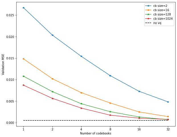
Here, d=64 was fixed, as this was sufficient for optimal performance in the no-VQ condition. Codebook size and number of codebooks was varied. As we can see, even with only two vectors per codebook, by using enough codebooks, we can achieve decent performance – actually better than with a single codebook with k=4096 in the previous experiment, even though using 32 codebooks we only have 64 vectors overall. Using larger codebooks, we can finally approach no-VQ performance.

There are different ways to interpret these results. Having “number of codebooks” on the x-axis is not really fair, since the models using larger codebooks of course have many more vectors overall. We can re-order the curves to have “total number of codebook vectors” on the x-axis:

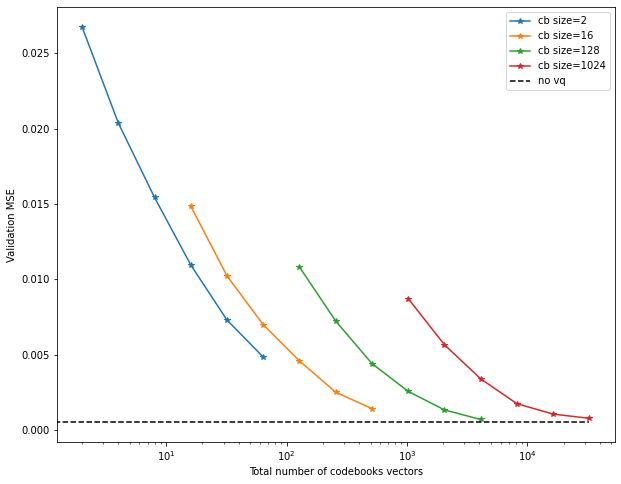
This is simply k * number_of_codebooks. This now seems to imply that using many smaller codebooks is actually more efficient in terms of performance. So is the answer to just use a huge number of size-2 codebooks? Not really. Recall that, at the end of the day, our main concern may be the degree of compression of the data, i.e. bit depth. 32 codebooks of size 2 may have 64 vectors overall, but the number of bits here is also 32 – one bit per codebook. On the other hand, a single codebook of size 64 only requires 6 bits. Thus, it may be a better idea to sort the x-axis by number of bits required:

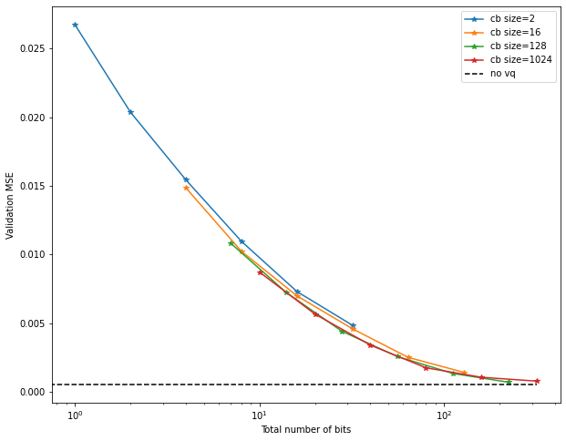
This reveals yet a different picture – it seems to barely matter what combination of codebook size and number we use to achieve a given number of bits! If anything, this implies that larger codebooks perform slightly better. Another striking feature is the very clean functional form – looks like a power law could be a good fit, for example. Using this, it may be possible to predict in advance how many bits would be required to achieve a certain performance.
Finally, we can also use “possible number of quantizations” for the x-axis. For example, as mentioned earlier, two codebooks of size 1024 allow for around one million different quantizations.

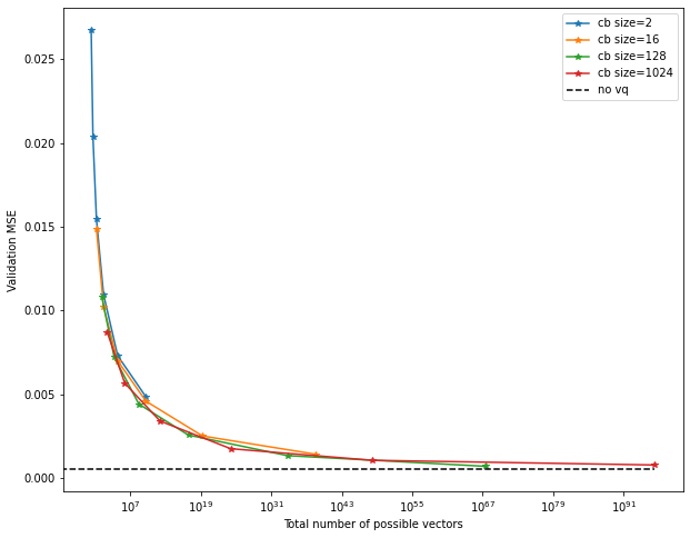
This looks similar to the previous plot, and that is no surprise – it turns out, the number of bits is just the (base-2) logarithm of the number of quantizations! As such, this is really just a re-scaling of the x-axis.

What About The Image Size?

To finish up, here is one more experiment: Recall that there are two ways to increase the overall number of bits: Increasing bit depth, or increasing the size of the encoded image. I wanted to see how the two relate, so I trained another set of models. These have basically the same architecture, but I cut off one set of layers to stop already at a resolution of 8x8. Results are shown below:

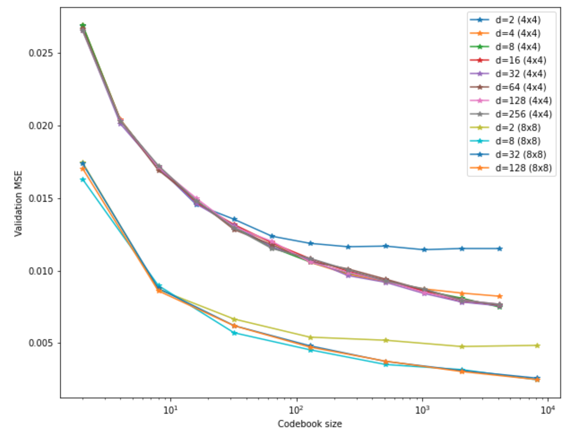
Here, I only tested the regular VQ-VAE, i.e. a single codebook, but varying number of entries k. This implies that, with the same codebook size, the 8x8 models perform better. But, of course, this is once again not a fair comparison: At the same bit depth (related directly to k), the 8x8 models have four times as many vectors in their latent space, and thus use four times more bits. We can once again equalize the x-axis by number of bits, this time for the whole encoded image:

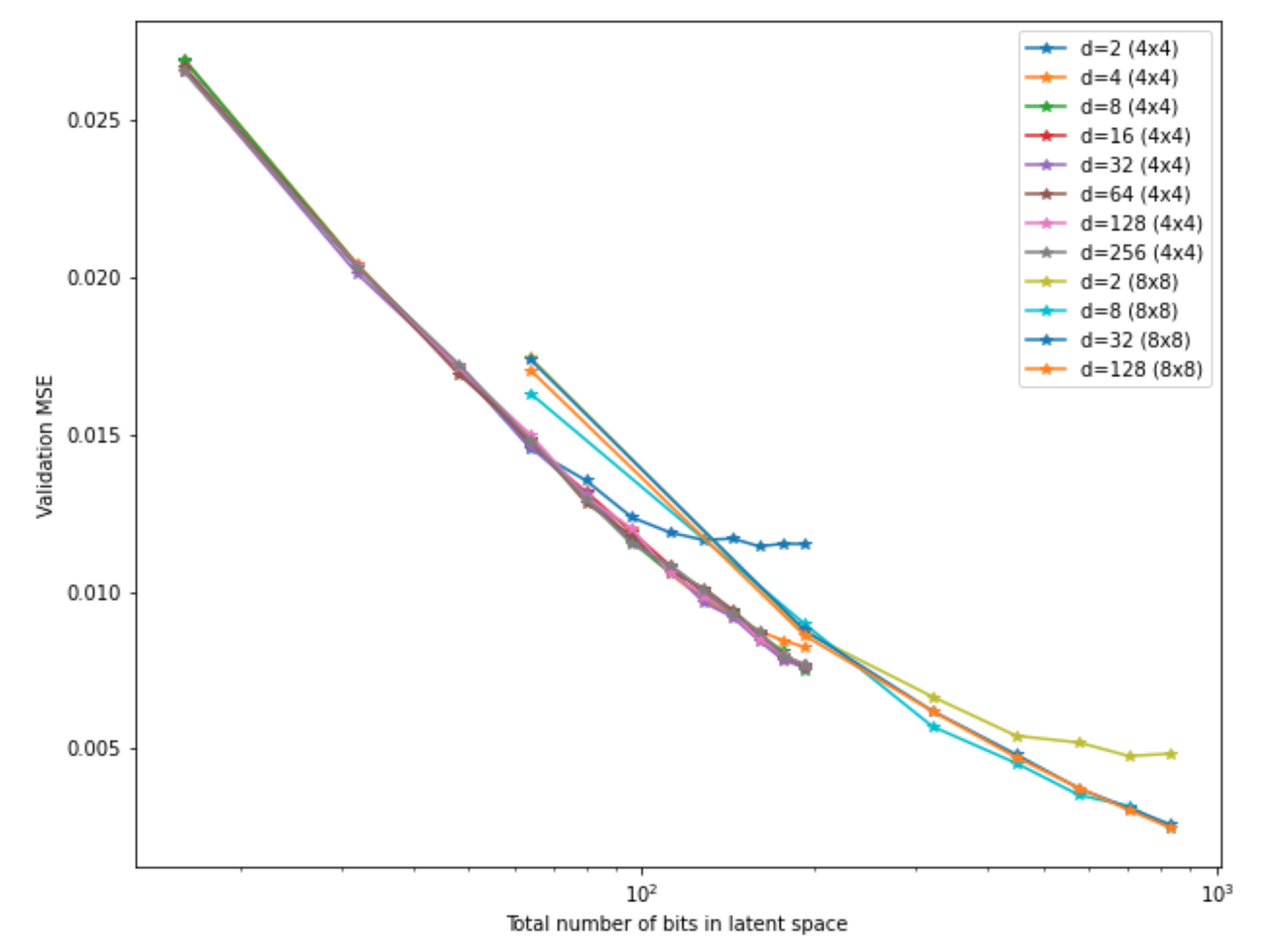
Looks like the 8x8 models actually perform worse! This once again shows how important it is to use the correct information on the axes. Of course, this could just be a quirk of the architecture design, since the 8x8 models simply have fewer layers, which could lead to weaker performance. This is not supposed to be an exhaustive test – I just wanted to showcase all the different factors we can vary.

Conclusion

We have seen that the number of bits in the latent space is key for good performance with VQ-VAEs. With a single codebook, it can be difficult to achieve higher bit rates, as these might require too many codebook vectors to be feasible. Residual vector quantization provides an interesting workaround; they seem to be a good option to achieve close-to-non-VQ performance. It remains to be seen whether such results generalize to more complex datasets and architectures. Here, other factors may start playing a confounding role, or more complex loss functions than MSE may not show the same predictable behavior. Still, it can be reassuring to see such clear and consistent behavior in the context of deep learning, where we often feel like we arestumbling through the dark when looking for improvements to our models.